Orthogonal Curvilinear Coordinates

Imagine that you need to numerically solve a differential equation, let’s say the Poisson’s equation, \(\nabla^2\phi=-\rho/\epsilon_0\), on an arbitrary curve. You can easily accomplish this using the Finite Difference Method, if (and this is a big if) the curve is aligned with one of the coordinate axes. If it’s not, like the curve shown in Figure 1, then you can derive the numerical scheme using the Finite Volume method. But this second approach is cumbersome. The scheme will be more complex since it will depend on two or three variables. Not only will this complicate the coding, it will also make the physical interpretation of the solution (which varies with the distance along the line) more difficult.
General orthogonal curvilinear coordinate system
So is there another option? We said in the introductions that the Finite Difference method can be used if the curve is aligned with a coordinate axis. So, why can’t we just define a new set of coordinates such that our curve becomes one of them?
Turns out we can – and this is the motivation for working in general orthogonal curvilinear coordinates. The difference between a general curvilinear system and the Cartesian one is that the axes orientation and scaling changes with the spatial position. But despite this, the axes always remain orthogonal. This is where the “orthogonal” part comes from (there are also non-orthogonal systems but those are more complicated to derive). You are already familiar with two curvilinear systems: the cylindrical and the spherical coordinates. In this post we will derive the math governing such systems. We will use it in a follow up post to develop the general curvilinear potential solver.

Scale Factors and Unit Vectors
Consider the position vector at some point in space. In the Cartesian coordinates, the position vector is given by \( \mathbf{r}=x\mathbf{i}+y\mathbf{j}+z\mathbf{k}\). To be more general, we define the vector as \( \mathbf{r}=x_1\mathbf{i}_1 + x_2\mathbf{i}_2 + x_3\mathbf{i}_3\). Now assume that at this point we have another orthogonal coordinate system \((u_1, u_2, u_3)\) such that \(u_i=u_i(x_1,x_2,x_3)\). Similarly, a reverse relationship also exists, \( x_i=x_i(u_1,u_2,u_3)\).
In order to define vector operators in this new coordinate system, we need to determine how the position vector changes with a change in this new coordinate system. The differential displacement in the \(u_1\) direction is given by
$$
\displaystyle d\mathbf{r}_1 = \frac{\partial \mathbf{r}}{\partial u_1} du_1 = \left[\frac{\partial x_1}{\partial u_1}\mathbf{i}_1 + \frac{\partial x_2}{\partial u_1}\mathbf{i}_2 + \frac{\partial x_3}{\partial u_1}\mathbf{i}_3\right] du_1
$$
The magnitude of this vector is \(|d\mathbf{r}_1| = |\partial \mathbf{r}/\partial u_1|du_1 = h_1du_1\). The \(h_1=|\partial \mathbf{r}/\partial u_1|\) term is called a scale factor. It relates the actual displacement in a given coordinate direction to the magnitude of the change of that coordinate.
With these definitions, we can define the unit vector in the \(u_1\) direction (basis vector),
$$
\displaystyle\mathbf{e}_1=\frac{d\mathbf{r}_1}{|d\mathbf{r}_1|}=\frac{1}{h_1}\frac{\partial \mathbf{r}}{\partial u_1}
$$
This expression can be rewritten as
$$
\displaystyle h_1\mathbf{e}_1 = \frac{\partial \mathbf{r}}{\partial u_1}
$$
When both sides of the equations are squared (dot product), we obtain an expression for the magnitude of the scale factor,
$$
\displaystyle h_1 =\sqrt{\left(\frac{\partial x_1}{\partial u_1}\right)^2 + \left(\frac{\partial x_2}{\partial u_1}\right)^2 + \left(\frac{\partial x_3}{\partial u_1}\right)^2}
$$
Of course, similar expressions exist in the two other directions.
Example: Scaling Factors in the Cylindrical Coordinate System
To demonstrate how this works, let’s consider the cylindrical coordinate. In these coordinates, \((u_1,u_2,u_3)=(r,\theta,z)\). With \((x_1,x_2,x_3)=(x,y,z)\) we have the following transformation \(x=r\cos\theta\), \(y=r\sin\theta\), and \(z=z\). Then
$$ \begin{array}{rcl}h_1&=&h_r=\sqrt{\cos^2\theta +\sin^2\theta + 0} = 1 \\ h_2&=&h_\theta = \sqrt{r^2\sin^2\theta + r^2\cos^2\theta} = r \\ h_3 &=& h_z = 1\end{array}$$
This implies that in cylindrical coordinates a differential displacement is given by \(d\mathbf{r} = d r\mathbf{e}_r + r d\theta\mathbf{e}_\theta + dz \mathbf{e}_z\)
Derivatives of Unit Vectors
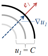 We will next derive two important sets of relationships that deal with derivatives of coordinates and unit vectors. First, consider the expression \(\nabla u_i\). Since \(u_i\) is a coordinate, regions with constant \(u_i\) define isosurfaces in our 3D domain. This value changes only in the direction normal to these isosurface, i.e. the direction of the coordinate basis vector. This concept is illustrated in the image to the right. Hence we have
$$\displaystyle \nabla u_i = \displaystyle \frac{\partial u_i}{\partial\mathbf{r}}=\frac{1}{h_i}\mathbf{e}_i$$
This expression is just another form (inverse) of the scale factor definition given in the previous section.
We next derive expressions for derivatives of unit vectors of form \(\mathbf{e}_p\cdot (\partial \mathbf{e}_q /\partial u_r)\). Consider the second derivative
$$
\displaystyle \frac{\partial^2\mathbf{r}}{\partial u_2 \partial u_1} = \frac{\partial}{\partial u_2}\left(\mathbf{e}_1h_1\right)=\frac{\partial \mathbf{e}_1}{\partial u_2} h_1 + \mathbf{e}_1 \frac{\partial h_1}{\partial u_2}
$$
Similarly, by inverting the order of differentiation, we obtain
$$
\displaystyle \frac{\partial^2\mathbf{r}}{\partial u_1 \partial u_2} = \frac{\partial}{\partial u_1}\left(\mathbf{e}_2h_2\right)=\frac{\partial \mathbf{e}_2}{\partial u_1} h_2 + \mathbf{e}_2 \frac{\partial h_2}{\partial u_1}
$$
Since the order of differentiation does not matter, the two expressions are equal. We set them to each other, and also dot both sides with \(\mathbf{e}_1\) to obtain
$$
\begin{array}{rcl}
\displaystyle \mathbf{e}_1\cdot\frac{\partial \mathbf{e}_1}{\partial u_2} h_1 + \mathbf{e}_1\cdot\mathbf{e}_1 \frac{\partial h_1}{\partial u_2} &=& \displaystyle\mathbf{e}_1 \cdot\frac{\partial \mathbf{e}_2}{\partial u_1} h_2 + \mathbf{e}_1\cdot\mathbf{e}_2 \frac{\partial h_2}{\partial u_1}\\[12pt]
\displaystyle 0 + \frac{\partial h_1}{\partial u_2} &=& \displaystyle\mathbf{e}_1\cdot\frac{\partial \mathbf{e}_2}{\partial u_1} h_2 + 0\\
\end{array}
$$
The first term on the LHS vanishes since a gradient is by definition normal to the surface of constant value which is what a basis vector gives us. The last term on the RHS also vanishes since the coordinate system is orthogonal, i.e. \(\mathbf{e}_1\cdot\mathbf{e}_2 = \mathbf{e}_2\cdot\mathbf{e}_3=\mathbf{e}_3\cdot\mathbf{e}_1=0\).
Finally,
$$
\displaystyle
\mathbf{e}_1\cdot \frac{\partial \mathbf{e}_2}{\partial u_1} = \frac{\partial}{\partial u_1}\left(\mathbf{e}_1\cdot\mathbf{e}_2\right) – \frac{\partial \mathbf{e}_1}{u_1}\cdot \mathbf{e}_2 = 0 – \frac{\partial \mathbf{e}_1}{u_1}\cdot \mathbf{e}_2
$$
again by orthogonality. We thus have
$$
\displaystyle
\mathbf{e}_2 \cdot \frac{\partial \mathbf{e}_1}{u_1} = – \frac{1}{h_2}\frac{\partial h_1}{\partial u_2}
$$
These expression can be summarized in a general form as
$$
\begin{array}{rcll}
\mathbf{e}_p\cdot\dfrac{\partial \mathbf{e}_q}{\partial u_p} &=& \dfrac{1}{h_q}\dfrac{\partial h_p}{\partial u_q} &\qquad p\ne q\\[12pt]
\mathbf{e}_q\cdot\dfrac{\partial \mathbf{e}_p}{\partial u_p} &=& -\dfrac{1}{h_q}\dfrac{\partial h_p}{\partial u_q} &\qquad p\ne q\\[12pt]
\mathbf{e}_p\cdot\dfrac{\partial \mathbf{e}_p}{\partial (\cdot)} &=& 0 &\qquad p\ne q \text{ or } p=q\\[12pt]
\end{array}
$$
Gradient
The first vector operator we define is the gradient. The gradient is given by
$$ \begin{array}{rcl}\nabla \mathbf{f} &=& \displaystyle \mathbf{i}_1 \frac{\partial f}{\partial x_1} + \mathbf{i}_2 \frac{\partial f}{\partial x_2} + \mathbf{i}_3 \frac{\partial f}{\partial x_3} \\[12pt] &=& \displaystyle \mathbf{i}_1 \left(\frac{\partial f}{\partial u_1}\frac{\partial u_1}{\partial x_1} + \frac{\partial f}{\partial u_2}\frac{\partial u_2}{\partial x_1} + \frac{\partial f}{\partial u_3}\frac{\partial u_3}{\partial x_1}\right) + \mathbf{i}_2 \left(\frac{\partial f}{\partial u_1}\frac{\partial u_1}{\partial x_2} + \frac{\partial f}{\partial u_2}\frac{\partial u_2}{\partial x_2} + \frac{\partial f}{\partial u_3}\frac{\partial u_3}{\partial x_2}\right) + \mathbf{i}_3 \Big(\dots\Big) \\[12pt] &=& \displaystyle \frac{\partial f}{\partial u_1} \nabla u_1 + \frac{\partial f}{\partial u_2}\nabla u_2 + \frac{\partial f}{\partial u_3}\nabla u_3 \end{array}$$
By substituting \(\nabla u_j = \mathbf{e}_j/h_j\) we obtain the general expression for the gradient,
$$ \displaystyle \nabla \mathbf{f} = \frac{1}{h_1}\frac{\partial f}{\partial u_1} \mathbf{e}_1 + \frac{1}{h_2}\frac{\partial f}{\partial u_2} \mathbf{e}_2 + \frac{1}{h_3}\frac{\partial f}{\partial u_3} \mathbf{e}_3$$
Gradient in Cylindrical Coordinates
As an example, using the previously calculated scale factors, the gradient in cylindrical coordinates is given by
$$\displaystyle \nabla f|_{cyl} = \frac{\partial f}{\partial r} \mathbf{e}_r + \frac{1}{r}\frac{\partial f}{\partial \theta} \mathbf{e}_\theta + \frac{\partial f}{\partial z} \mathbf{e}_z$$
Derivation using vector transformation
As a little aside, the steps given above are just one of many different approaches for obtaining the gradient. See the references listed below for additional approaches. As an example of an alternative, using the method in [1], we can obtain the same expression by considering vector transformation. Using the index notation, the gradient operator is written as
$$\displaystyle (\nabla f)_i = \frac{\partial}{\partial x_i}\phi$$
By chain rule we have
$$\displaystyle \frac{\partial}{\partial x_i}\phi = \frac{\partial u_j}{\partial x_i}\frac{\partial}{\partial u_j}f$$
We can next multiply and divide the right hand side by \(h_j\). In writing proofs using the index notation, it is a common practice to perform substitutions like this to come up with terms that correspond to some other previously defined terms, or to terms that will allow us to utilize identities. In this case, this multiplication gives us the vector transformation,
$$\displaystyle \begin{array}{rcl}(\nabla f)_i &=& \displaystyle h_j \frac{\partial u_j}{\partial x_i} \frac{1}{h_j} \frac{\partial}{\partial u_j}f\\ &=& a_{ji}(\nabla’ f)_j\end{array} $$
and hence gradient in the new coordinate system is defined by
$$\displaystyle \left(\nabla’ f\right)_j = \frac{1}{h_j}\frac{\partial}{\partial u_j} f$$
which is the same as the expression given above.
Divergence
Divergence is computed directly from the definition of the gradient,
$$\displaystyle \nabla \cdot \mathbf{f} = \left(\frac{\mathbf{e}_1}{h_1}\frac{\partial}{\partial u_1} + \frac{\mathbf{e}_2}{h_2}\frac{\partial }{\partial u_2} + \frac{\mathbf{e}_3}{h_3}\frac{\partial}{\partial u_3}\right)\cdot\left(\mathbf{e}_1f_1 + \mathbf{e}_2f_2 + \mathbf{e}_3f_3\right)$$
Evaluating just the first (\(\mathbf{e}_1 f_1\)) term we get
$$\displaystyle (\nabla \cdot \mathbf{f})_1 = \frac{\mathbf{e}_1}{h_1} \frac{\partial}{\partial u_1}\left(\mathbf{e}_1f_1\right) + \frac{\mathbf{e}_2}{h_2}\frac{\partial}{\partial u_2} \left(\mathbf{e}_1f_1\right) + \frac{\mathbf{e}_3}{h_3}\frac{\partial}{\partial u_3} \left(\mathbf{e}_1f_1\right)$$
We next expand each of the terms above, starting with the first one,
$$\begin{array}{rcl} \displaystyle \frac{\mathbf{e}_1}{h_1} \frac{\partial}{\partial u_1}\left(\mathbf{e}_1f_1\right) &=& \displaystyle \frac{\mathbf{e}_1}{h_1} \frac{\partial \mathbf{e}_1}{\partial u_1}f_1 + \frac{\mathbf{e}_1}{h_1} \frac{\partial f_1}{\partial u_1}\mathbf{e}_1 \\[12pt] &=& \displaystyle\frac{1}{h_1} \frac{\partial f_1}{\partial u_1}\end{array}$$
since the first term is zero as noted above in the section on derivatives of unit vectors.
For the second term we get
$$\begin{array}{rcl} \displaystyle \frac{\mathbf{e}_2}{h_2} \frac{\partial}{\partial u_2}\left(\mathbf{e}_1f_1\right) &=& \displaystyle \frac{\mathbf{e}_2}{h_2} \frac{\partial \mathbf{e}_1}{\partial u_2}f_1 + \frac{\mathbf{e}_2}{h_2} \frac{\partial f_1}{\partial u_2}\mathbf{e}_1 \\[12pt] &=& \displaystyle\frac{1}{h_2}\frac{1}{h_1} \frac{\partial h_2}{\partial u_1}f_1\end{array}$$
since \(\mathbf{e}_2\cdot\mathbf{e}_1=0\) by orthogonality, and the previously derived identity is used for the other term.
We obtain a similar expression for the last term,
$$\begin{array}{rcl} \displaystyle \frac{\mathbf{e}_3}{h_3} \frac{\partial}{\partial u_3}\left(\mathbf{e}_1f_1\right) &=& \displaystyle \frac{\mathbf{e}_3}{h_3} \frac{\partial \mathbf{e}_1}{\partial u_3}f_1 + \frac{\mathbf{e}_3}{h_3} \frac{\partial f_1}{\partial u_3}\mathbf{e}_1 \\[12pt] &=& \displaystyle\frac{1}{h_3}\frac{1}{h_1} \frac{\partial h_3}{\partial u_1}f_1\end{array}$$
Combining these pieces together, we get an expression for the first component of divergence,
$$\displaystyle \left(\nabla \mathbf{f}\right)_1 = \frac{1}{h_1}\frac{\partial f_1}{\partial u_1} + \frac{1}{h_2h_1}\frac{\partial h_2}{\partial u_1}f_1 + \frac{1}{h_1h_3}\frac{\partial h_3}{\partial u_1}f_1$$
or, in a more compact way,
$$\displaystyle \left(\nabla \mathbf{f}\right)_1 = \frac{1}{h_1h_2h_3}\frac{\partial}{\partial u_1}\left(f_1h_2h_3\right)$$
The other two terms are derived in a similar fashion, giving us the expression for divergence
$$\displaystyle \nabla \mathbf{f} = \frac{1}{h_1h_2h_3}\left[\frac{\partial}{\partial u_1}\left(f_1h_2h_3\right) + \frac{\partial}{\partial u_2}\left(f_2h_3h_1\right) + \frac{\partial}{\partial u_3}\left(f_3h_1h_2\right)\right]$$
As an example, in the cylindrical coordinates we have
$$\begin{array}{rcl}\displaystyle \left(\nabla \mathbf{f}\right)|_{cyl} &=& \displaystyle\frac{1}{r}\left[\frac{\partial}{\partial r}\left(rf_r\right) + \frac{\partial}{\partial \theta}\left(f_\theta\right) + \frac{\partial}{\partial u_z}\left(rf_z\right)\right] \\[12pt] &=& \displaystyle\frac{1}{r}\frac{\partial }{\partial r}\left(rf_r\right) + \frac{1}{r}\frac{\partial f_\theta}{\partial \theta} + \frac{\partial f_z}{\partial u_z}\end{array}$$
The Laplace Operator
The Laplacian is a combination of a divergence and a gradient, i.e. \(\nabla^2 f = \nabla\cdot\nabla f = \nabla \cdot \mathbf{g}\) where \(\mathbf{g}=\nabla f\). We have
$$\displaystyle\begin{array}{rcl}\nabla^2 f &=& \displaystyle \sum_{j=1}^3\frac{1}{h_1h_2h_3}\frac{\partial}{\partial u_j}\left(\frac{h_1 h_2 h_3}{h_j}f_j\right) \\ &=& \displaystyle \sum_{j=1}^3\frac{1}{h_1h_2h_3}\frac{\partial}{\partial u_j}\left(\frac{h_1h_2h_3}{h_j}\frac{1}{h_j}\frac{\partial f}{\partial u_j}\right)\end{array}$$
In the expanded form, this is
$$\displaystyle \nabla^2 f = \frac{1}{h_1h_2h_3}\left[\frac{\partial}{\partial u_1} \left(\frac{h_2h_3}{h_1}\frac{\partial f}{\partial u_1}\right) + \left(\frac{h_1h_3}{h_2}\frac{\partial f}{\partial u_2}\right) + \left(\frac{h_1h_2}{h_3}\frac{\partial f}{\partial u_3}\right) \right]$$
Again, using the previously defined scale factors, we find the Laplacian in cylindrical coordinates,
$$\displaystyle \begin{array}{rcl} \nabla^2 f |_{cyl} &=& \displaystyle \frac{1}{r}\left[\frac{\partial}{\partial r}\left(r\frac{\partial f}{\partial r}\right)\right] + \frac{1}{r}\left[\frac{\partial}{\partial \theta}\left(\frac{1}{r}\frac{\partial f}{\partial \theta}\right)\right] + \frac{1}{r}\left[\frac{\partial}{\partial z}\left(r\frac{\partial f}{\partial z}\right)\right] \\[12pt] &=& \displaystyle \frac{1}{r}\left[\frac{\partial}{\partial r}\left(r\frac{\partial f}{\partial r}\right)\right] + \frac{1}{r^2}\frac{\partial^2f}{\partial \theta^2} + \frac{\partial^2f}{\partial z^2} \end{array}$$
Curl
The final piece that is missing in the arsenal of vector calculus is the curl. Again using the definition of divergence we have
$$\displaystyle \nabla \times \mathbf{f} = \left(\mathbf{e}_1\frac{1}{h_1}\frac{\partial}{\partial u_1} + \mathbf{e}_2\frac{1}{h_2}\frac{\partial}{\partial u_2} + \mathbf{e}_3\frac{1}{h_3}\frac{\partial}{\partial h_3}\right)\times \left(\mathbf{e}_1 f_1+\mathbf{e}_2 f_2 + \mathbf{e}_3 f_3\right)$$
which we can evaluate using the standard determinant approach, i.e.,
$$\nabla \times \mathbf{f} = \dfrac{1}{h_1h_2h_3} \left|\begin{array}{ccc}h_1\mathbf{e}_1 & h_2\mathbf{e}_2 & h_3 \mathbf{e}_3 \\ \partial/\partial u_1 & \partial/\partial u_2 & \partial/\partial u_3 \\ h_1f_1 & h_2f_2 & h_3f_3\end{array}\right|$$
By plugging in the scale factors, we find that in the cylindrical coordinates,
$$\begin{array} {rcl}(\nabla \times \mathbf{f})|_{cyl} &=& \dfrac{1}{r} \left|\begin{array}{ccc}\mathbf{e}_r & r\mathbf{e}_\theta & \mathbf{e}_z \\ \partial/\partial r & \partial/\partial \theta & \partial/\partial z \\ f_r & rf_\theta & f_z\end{array}\right| \\ &=& \displaystyle \frac{1}{r}\left(\frac{\partial f_z}{\partial \theta} -r\frac{\partial f_\theta}{\partial z}\right) \mathbf{e}_r – \left(\frac{\partial f_z}{\partial r} – \frac{\partial f_r}{\partial z}\right) \mathbf{e}_\theta + \frac{1}{r}\left(\frac{\partial \left(rf_\theta\right)}{\partial r} – \frac{\partial f_r}{\partial \theta}\right)\mathbf{e}_z \end{array}$$
You will find additional definitions and the forms of these vector operators in spherical coordinates on the Wikipedia page Del in Cylindrical and Spherical Coordinates.
References
This article was based primarily on author’s notes from MAE 221, Fluid Mechanics, taught by Dr. Michael Myers at the George Washington University in the Fall of 2008. It was a tough class but definitely worth it! Additional useful resources include:
- Orthogonal, curvilinear coordinates, author unknown. This document provides a very nice treatment of coordinate transformation using the index notation. Unfortunately, I could no longer find it online. Please contact me if you have the link, or if you would like my copy of this document.
- Orthogonal Curvilinear Coordinates from Calculus III by Dr. Will Sutherland, Queen Mary University of London
- Orthogonal Curvilinear Coordinates by Dr. Phyllis R. Nelson, ECE, Cal Poly Ponoma
- Orthogonal Curvilinear Coordinates by Prof. H.M. Atassi, MAE, University of Notre Dame
- Ortogonal Curvilinear Coordinates, Prof. Baron Peters, Chem. Eng, UC Santa Barbara
- Curvilinear Coordinates by Prof. Frederick Stern, Intermediate Mechanics of Fluids, U. Iowa
- Curvilinear Coordinates on Wikipedia (a very generalized, math-heavy treatment)
Feel free to leave a comment if you have any questions or comments. I did my best to check all equations, but since this article is bit math heavy, it is possible that something slipped through the cracks. Let me know if you find any mistakes.
please give the answer for laplace operators in orthogonal curvelinear co-ordinates and theirexplicit form in cartesion co-ordinates
Hi, you can find these online on Wikipedia:
http://en.wikipedia.org/wiki/Del_in_cylindrical_and_spherical_coordinates
How is it that
\(\nabla {u_i}=\frac{1}{h_i}\textbf{e}_i\)
Hi,
you solve the case in which you know the relationship between axes.
But I am interested in the plot you made, where the axes are varying along an arbitrary curve.
How should I approach this case? (I only need h1, h2 and h3)
thanks
Hi ,
Pls tell the answer for Show that spherical co- ordinate system is orthogonal
How it is that
\(\nabla u_i = frac{1}{h_i} \textbf{e}_i\)
How is it that
\(\nabla u_i = \frac{1}{h_i}\textbf{e}_i\)
del ui points in the same direction as ui and is: (say del 2)
unit in del 2 direction = (del 1 X del 3) / abs (del 1 X del 3)
unit in d/du2 direction = (dR/du2)/abs (dR/du2) R denotes vector. Or dR/ds. dR/ds = (dR/du2)/abs(dR/du2
s is arc length