Current Density Limit

One difference between ion thrusters and Hall Effect thrusters is that ion thrusters are space charge limited devices. The region between the grids of the ion thruster is occupied solely by ions, and is thus subject to the Child Langmuir law. This law, given by
$$ J_{CL}=\frac{4}{9}\epsilon_0 \sqrt{\frac{2q}{m}} \frac{|\Delta \phi|^{1.5}}{(\Delta x)^2} $$
gives the maximum current density that can be extracted between two planar electrodes $latex Delta x$ apart and having potential difference of $latex Delta phi$. To illustrate the concept, I put together a small Matlab program for my propulsion class at the George Washington University. The program (current.m) is given below. It simulates flow of singly-charged Xenon ions, emitted from an anode at x=0, and moving towards a cathode located 1cm away, with potential difference of 100V. For this configuration, the Child Langmuir law predicts maximum current density of 0.0477 A/m2.
% Simulation to study Child Langmuir current density limit
% For more see:
% https://www.particleincell.com/blog/2014/current-density

more off;			%turn off pagination in Octave

%physical constants
AMU = 1.6605e-27;	%atomic mass in kg
E = 1.6022e-19;		%elementary charge in Coulomb
EPS0 = 8.8542e-12;	%permittivity of free space F/m
ME = 9.1094e-31;	%electron mass

%set boundaries
phi_left = 0;
phi_right = -100;
x_left = 0;
x_right = 0.01;

%compute mesh parameters
nx = 100;				%number of mesh nodes
delta_x = (x_right-x_left)/(nx-1);	%cell spacing, there are nx-1 cells

%set matrix data
A = zeros(nx);
A(1,1) = 1;		%fixed potential at left
A(nx,nx) = 1;		%fixed potential at right
for i=2:nx-1
	%finite difference stencil for second derivative
	A(i,i-1) = 1;
	A(i,i) = -2;
	A(i,i+1) = 1;
end


%ion data
ion_mass = 131.3*AMU;
ion_charge = 1*E;

%time data
delta_t=0.5*delta_x/sqrt(2*ion_charge/ion_mass*(abs(phi_right-phi_left))) %time step
it_max = 3000;		%number of time steps


%injection current
j_CL = (4/9)*EPS0*sqrt(2*ion_charge/ion_mass)*(abs(phi_right-phi_left))^1.5/(x_right-x_left)^2;
I = 1*j_CL		%this is also current density due to unit length in y and z
np_inject = 10;	%number of particles to inject per time step
ion_spwt = I*delta_t/(ion_charge*np_inject);	%number of actual particles per macroparticle

%initialize
part_count = 0;		%number of particles
efield = zeros(nx,1);

%main loop
for it=1:it_max

	%*** 1) generate new particles ***
	for p=1:np_inject		%inject particles
		%increment particle counter
		part_count=part_count+1;

		part_x(part_count) = 0;	%initial position
		part_v(part_count) = 0;	%initial velocity
		part_new(part_count) = 1;	%mark new particles

		%compute electric field at particle position
		fi = (part_x(part_count)-x_left)/delta_x + 1;
		i = floor(fi);
		di = fi-i;
		part_ef = efield(i)*(1-di)+efield(i+1)*(di);

		%rewind the velocity back by 0.5*delta_t, this part of the leapfrog scheme
		part_v(part_count) = part_v(part_count) - (ion_charge/ion_mass)*part_ef*0.5*delta_t;
	end

	%*** 2) compute field quantities***
	u = zeros(nx,1);
	count = zeros(nx,1);		%this field holds number of macroparticles
	for p=1:part_count
		%get particle mesh index
		fi = (part_x(p)-x_left)/delta_x + 1;
		i = floor(fi);
		di = fi-i;
		count(i) = count(i)+(1-di);
		count(i+1) = count(i+1)+ (di);

		u(i) = u(i)+(1-di)*part_v(p);
		u(i+1) = u(i+1)+ (di)*part_v(p);
	end
	den = ion_spwt*count/delta_x;	%divide by "volume"
	den(1) = den(1)* 2.0;			%only half area at boundaries
	den(nx) = den(nx)*2.0;

	%average velocity, make sure we don't divide by zero
	u(count~=0) = u(count~=0)./count(count~=0);
	u(count==0) = 0;
	j = den.*u*ion_charge;	%current density

	%*** 3) set charge density
	rho = den*ion_charge;

	%*** 4) solve potential ***
	b = -rho/EPS0*delta_x*delta_x;
	b(1) = phi_left;
	b(nx) = phi_right;
	phi = Ab;

	%*** 5) update electric field ***
	efield = -gradient(phi,delta_x);

	%*** 6) move particles ***
	for p=1:part_count
		%obtain electric field at the particle position
		fi = (part_x(p)-x_left)/delta_x + 1;
		i = floor(fi);
		di = fi-i;
		part_ef = efield(i)*(1-di)+efield(i+1)*(di);

		% set random delta_t for newly born particles
		if (part_new(p))
			dt = (1.0+1.0*rand())*delta_t;
			part_new(p) = 0;	%clear new particle flag
		else
			dt = delta_t;
		end

		%update particle velocity from F=m(dv/delta_t)=qE
		part_v(p) = part_v(p)+(ion_charge/ion_mass)*part_ef*dt;

		%update particle position
		part_x(p) = part_x(p)+part_v(p)*dt;

		%remove particles that crossed boundaries
		if (part_x(p)<x_left || part_x(p)>=x_right)
			%remove particle by replacing the current array data with the last
			part_x(p) = part_x(part_count);
			part_v(p) = part_v(part_count);
			part_new(p) = part_new(part_count);
			part_count=part_count-1;		%decrement particle counter
			p=p-1;		%also decrement current index to rescan this position
		end
	end

	%*** 7) output some diagnostics

	%plot results
	if (mod(it,25)==0 || it==it_max)
	disp(sprintf('it = %dt j_ave = %4.3g',it,mean(j(j~=0))));
		x_pos = [1:nx]*delta_x+x_left;
 		figure(1);
 		plot(x_pos,phi);
 		title('Potential');
 		figure(2);
 		plot(x_pos,efield);
 		title('Electric Field');
 		figure(3);
 		plot(x_pos,j,'-*');
 		title('Current Density');
 		axis([x_left,x_right, 0, 1.2*I]);
 		figure(4);
		plot(x_pos,u,'-*');
		title('Velocity');
		axis([x_left,x_right, -2000, 12000]);

		%for saving animation
		%filename=sprintf('v%05d.png',it);
		%print(filename);
		drawnow;
	end
end
Code Testing
First, we can make some simple sanity checks, by considering what happens if there is no electric field. This was done by commenting out the line to calculate electric field:
%*** 5) update electric field ***
%	efield = -gradient(phi,delta_x);
and changing the injection velocity to a non-zero value:
part_v(part_count) = 1000; %initial velocity
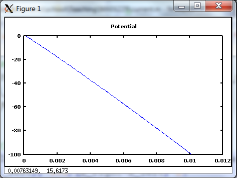
Figure 1 shows results for this case. As expected, the velocity remains constant and so does the injection current.
Results
Next, we can consider an actual simulation with the electric field enabled. For the first case, we set the injection current density to $latex 0.2 j_{CL}$ by using the following line
I = 0.2*j_CL %this is also current density due to unit length in y and z
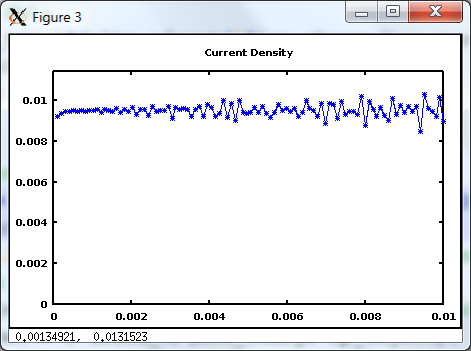
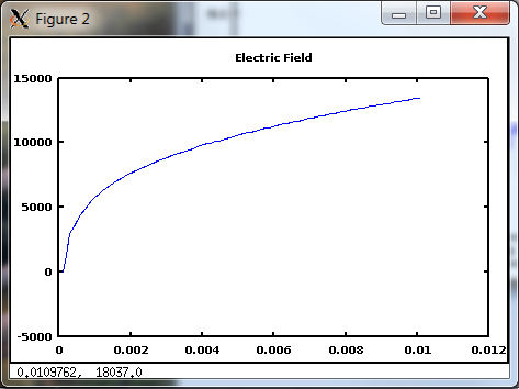
As shown in Figure 2, for this case the current density remains constant at the prescribed value of 0.0095 A/m2. The electric field and potential are also plotted.

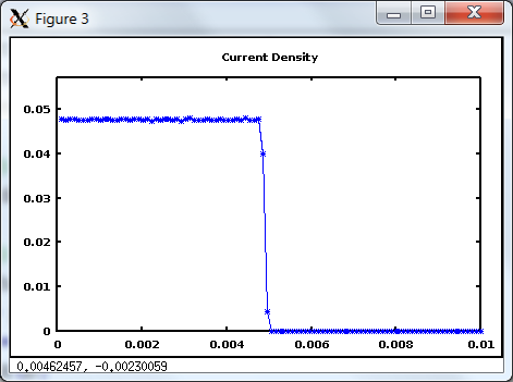
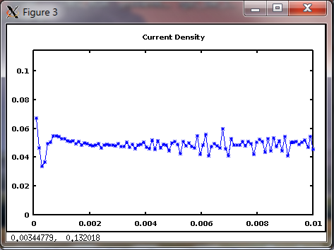
The results get more interesting once the injection current density exceeds the Child Langmuir law. Figure 3 shows these results for injection current of 2 J_CL. Once the discharge becomes space charge saturated, a negative electric field forms at the anode, which then prevents additional ions to enter the simulation. Only as many ions are allowed to pass as is needed to maintain the current density at the Child Langmuir limit.
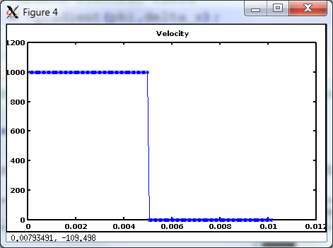
We can demonstrate this behavior further by giving ions a small initial velocity. This will cause them to travel a short distance from the injector electrode before being turned back. We can also visualize the dynamic behavior by creating an animation. To do this, I used the process described here to export png files for individual frames and then used ImageMagick to create the animated gif with the following commands:
$ find -name 'v*.png' -maxdepth 1 -exec convert {} -resize 400x400 small/{} ;
$ cd small
$ convert -delay 10 -loop 0 v*.png v_anim_small.gif
The figure below shows the average velocity. Negative value indicates that the majority of ions are moving in the opposite direction, towards the emitter electrode.