Starfish Tutorial Part 4: Steady State, Surface Flux, and Averaging

Introduction

This is part 4 of a five part tutorial on our plasma simulation code Starfish. In this part we continue the surface interaction topic introduced in step 3. More specifically, we will learn how to export surface properties, such as surface flux and deposition rate. We will also set up averaging to obtain averaged field properties. Let’s assume that we want to determine the rate with which the ions are arriving at the object, and also how much stuff is sticking to it. These are just two examples of surface (boundary) properties that can be exported from the simulation.

Steady State

But before we start discussing surface flux, we need to introduce the concept of steady state. Many computer simulation methods, especially ones based on kinetic approaches, such as PIC and DSMC, work by integrating simulation particles forward in time from some known initial state. The simulation will initially pass through a transient state in which the results are constantly changing and are not indicative of the final steady solution. As such, we need to wait until steady state to start collection cumulative data. Starfish automatically waits until steady state before starting to collect properties such as surface flux. This is an important point to note if you want to export cumulative data.

By default, the steady state is determined automatically. But you can also override it. As an example, here is a typical time command:

time>
<num_it>500</num_it>
<dt>5e-7</dt>
</time>

Here is one that tells the code to pretend the steady state is reached at iteration 100:

time>
<num_it>500</num_it>
<dt>5e-7</dt>
<steady_state>100</steady_state>
</time>

This second approach forces Starfish to turn on “steady-state” data collection at time step 100, regardless of whether the simulation has reached an actual steady state. This second approach is needed whenever time-variant sources are used or whenever the physical solution does not reach a real steady state. Such is the case in some types of plasma thrusters which, despite constant inlet propellant flow, reach only an oscillatory steady state due complex interactions between different species.

How is steady state determined?

So how does Starfish characterize steady state? Steady state simply means that the properties of interest are no longer changing. Let’s consider the typical gas flow governing equations. First we have the mass conservation:
$$\dfrac{\partial \rho}{\partial t} + \nabla\cdot(n\vec{u}) = 0$$
Here \(rho\) is the mass density. For steady state, we need the time dependent term on left to vanish. Clearly, one possible check is to iterate over the computational mesh and check the density at each node against the previous value. Disadvantage of this approach are the added memory requirements. Better approach is to consider the total mass, \(M\equiv = \int_v \rho \text{dV}\). With the mesh-based approach, \(M=\sum \rho_i V_i\), where we sum the density and the node volume over all nodes. Popular approach used in a number of PIC codes is to use the particles instead of the mesh and compare the number of simulation particles between two successive time steps. If the difference is smaller than some tolerance, the steady state is achieved:

if (abs((part_count-part_count_old)/(part_count))<tol) 
     steady_state = true;
else 
     part_count_old = part_count_old;

This approach is analogous if all particles have the same specific weight. If not, then the variable weight needs to be taken into account.

This approach works quite well in practice, but it checks only mass conservation. However, as we know, conservation of mass is just one of several governing equations that need to be satisfied by the flow. For instance, we also have the momentum equation,
$$\rho\left(\frac{\partial\vec{v}}{\partial t} + \vec{v}\cdot \nabla \vec{v} \right) = \vec{F}$$
So to be more accurate, we should also check the system momentum to make sure that
$$\dfrac{\partial L}{\partial t} \equiv \int_V \rho\frac{\partial|\vec{v}|}{\partial t} \text{dV} = 0$$.

Of course, we can get even more involved: for instance, the three components of linear momentum could be considered separately. We could also consider the total energy. However, from experience, these two checks are generally sufficient. Starfish uses these two checks to implement the following algorithm:

ratio_mass = (tot_mass - tot_mass_old)/tot_mass;
ratio_momentum = (tot_momentum - tot_momentum_old)/tot_momentum;
if (abs(ratio_mass)<1e-3 && abs(ratio_momentum)<1e-3)
     countown--;
else
     countdown = 5;
 
if (countdown<=0) steady_state = true;
 
tot_mass_old = tot_mass;
tot_momentum_old = tot_momentum_old;

In other words, the code waits until both mass and momentum change by less than 0.1% between time steps for 5 consecutive time steps. Once this happens, the steady state is reached. This algorithm works well for most situations, but as noted above, there may be some special cases when you will need to override it, and set the steady state manually.

Surface Flux

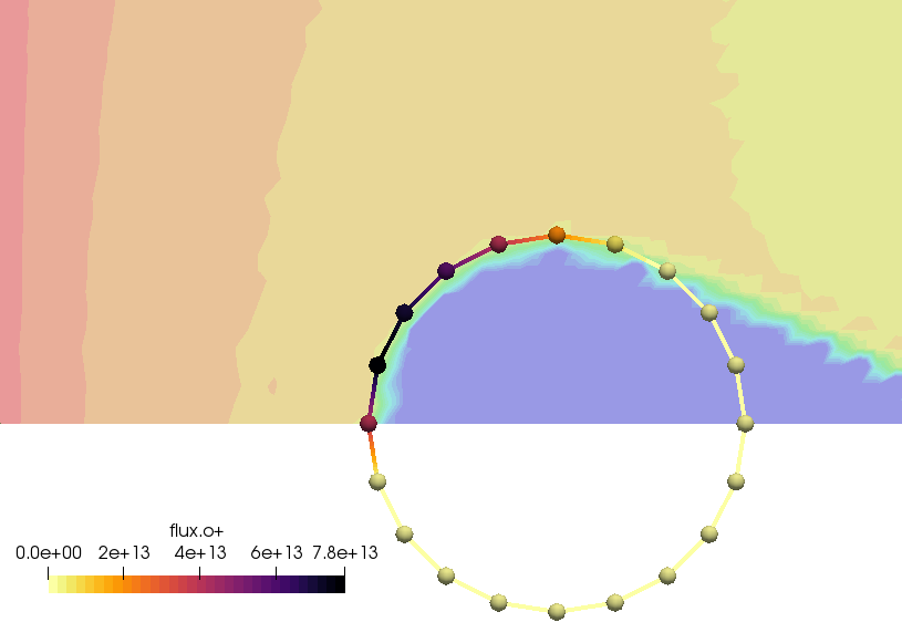
One thing that occurs once steady state is reached is that the code will start collecting information about particles hitting surfaces. This includes properties such as flux of individual materials, as well as the mass deposition rate, corresponding to the particles that stick (are absorbed) to the surface. We can output these properties by adding list of variables to the output statement,

<output type="boundaries" file_name="boundaries.dat" format="tecplot">
<variables>flux.o+, flux-normal.o+, deprate, depflux</variables>
</output>

Previously, the boundaries.dat file contained just the geometry of the cylinder. After this addition, the file will also contain four additional values corresponding to the number flux of oxygen ions and atoms (in #/m²/s), total mass flux summed over all materials (in kg/m²/s), and the mass deposition rate (in kg/s). These results are plotted below in Figure 1.

Data Averaging

Since results from kinetic codes are quite noisy, it is a good practice to average results over several time steps to get smoother plots, and to eliminate outlier data arising from statistical noise. This is done in Starfish with the averaging command. The syntax is

<!-- setup averaging -->
<averaging frequency="2">
<variables>phi,nd.o+,nd.o</variables>
</averaging>

The averaging starts automatically at steady state, and new data will be added every 2 time steps. The variables lines lists the variables to be averaged. Since averaging data adds a computational overhead, the code averages just the variables that are specified here. These averaged values are then exported using the standard output command, with the caveat that the averaged versions will have the base ending in “-ave”. For instance,

<!-- save results -->
<output type="2D" file_name="results/field.vts" format="vtk">
<scalars>phi, phi-ave, rho, nd.o+, nd.o, nd-ave.o+, nd-ave.o, t.o+, t.o</scalars>
<vectors>[efi, efj], [u.o+,v.o+], [u.o,v.o]</vectors>
</output>

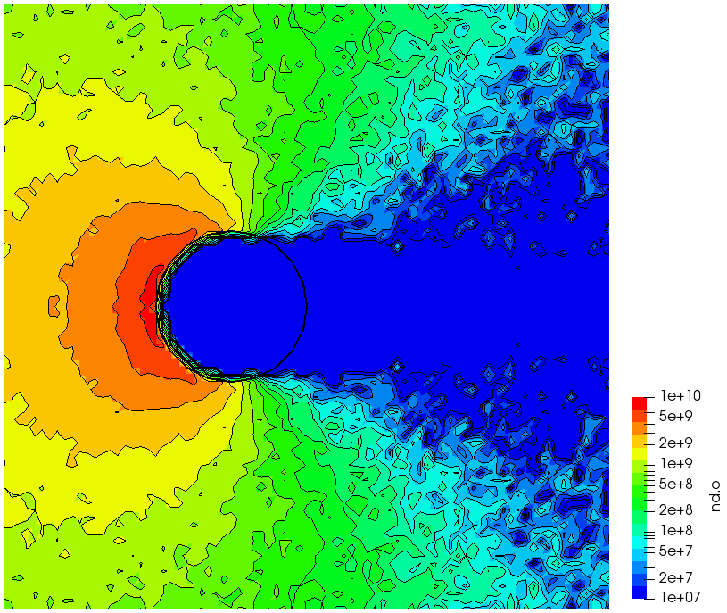
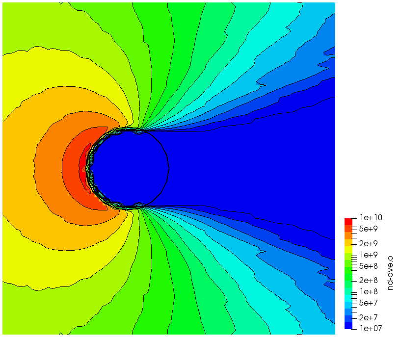
This command will output the following variables: instantaneous potential, averaged potential,
charge density, instantaneous ion and neutral density, averaged ion and neutral density, and time averaged temperature. Because of the way temperature is calculated (by collecting velocity samples), this data is automatically time averaged. Figure 2 below shows the differences.

Continue onto Part 5.