JWST Contamination Deposition Analysis

The James Webb Space Telescope (JWST) was launched in 2021 and has since stunned to world with amazing new images of deep space. These observations are partly due to the telescope operating in the infrared regime, unlike its “predecessor”, the Hubble Space Telescope. At IR wavelengths, the telescope can see through dust clouds to reveal previously hidden features. The IR regime however introduced a new challenge: needing to maintain all spacecraft components within the line of sight of the telescope extremely cold to prevent their thermal emissions from overwhelming the faint collected signal. As you are likely already aware, JWST accomplished this by splitting the satellite into two parts: a cold “observatory” facing deep space and the warm “spacecraft” facing the Sun. The interface was formed by the characteristic five layer sunshield. The resulting thermal profile introduced an interesting wrinkle from the contamination control and systems engineering perspectives. Despite water being found on most surfaces, and water also being one of the primary constituents of material released by outgassing, historically contamination analysts have not found themselves too concerned with water vapor. The reason is that at the low pressures found in space, water requires temperatures around 150K (-125C) to start freezing. Typical spacecraft utilize on-board heaters in conjunction with a possible “rotisserie” in the sunshine to maintain surfaces within a narrow band around the standard room temperature. The need to keep the observatory cold did not make it possible for JWST to achieve a similar thermal profile. Shortly post launch, the spacecraft was rotated into the operational orientation with the observatory side facing away from the Sun towards the deep space. Even prior to the sunshield deployment, the observatory already begins cooling due to being shadowed by the main spacecraft structure.
Due to adhering to surfaces, components with a large surface area – such as the sunshield – act as major sources of water. In the case of thin membranes, the water is expected to desorb relatively rapidly (within few days). Other components, such as composites and electronic boxes, become long-term outgassers of water and other contaminants. The production rate of both decays with time as the source becomes depleted. At the same time, the observatory continues to cool down. Water, especially in the ice form, can lead to a number of issues. Ice changes surface thermal emission profiles and also scatters light. It can also lead to difficulties in deploying mechanical actuators. JWST system engineers were clearly interested in understanding how much water and other contaminants can be expected to deposit onto the observatory. The answer was essentially driven by the race between cooling and source depletion. Are the sources becoming depleted faster than the surfaces are cooling? Answering this question required inputs from multiple engineering disciplines, including mechanical, thermal and contamination control. Particle in Cell Consulting (PIC-C) assisted NASA in answering this question for contamination. The goal of this article is to summarize this work. All information provided here comes from our 2022 SPIE Optics and Photonics paper, “Numerical study of water ice and molecular contamination build up during JWST deployment” coauthored by me and my assistant at the time Marc Laugharn, as well as Michael Woronowicz, Kelly Henderson-Nelson, Christopher May, Eve Wooldridge from NASA Goddard. The paper goes into much more detail than what is given here. The analysis was performed using our kinetic code CTSP.
Simulation Inputs
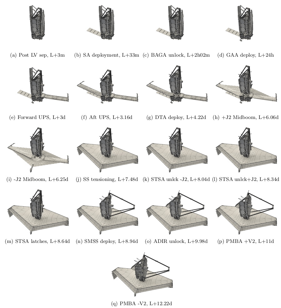
Our objective was to model the ice and contaminant build up during the first 180 days in space that corresponded to the commissioning phase. What made this analysis so challenging was needing to consider the variation in surface configuration due to the unfolding of the “origami” telescope as necessitated by the limited real estate inside a launch vehicle fairing. Figure 1 visualizes the 17 considered configurations. These configurations were provided to us in the Thermal Synthesizer System (TSS) format. It uses an assembly of analytical shapes such as cylinders, cones, rectangles, and so on to describe the geometry. Each shape can be individually rotated or translated, with similar transformations as well as mirroring also applicable at the assembly level. These transformations can be described using analytical expressions utilizing variables. A lot of initial work involved developing a parser for this file format.
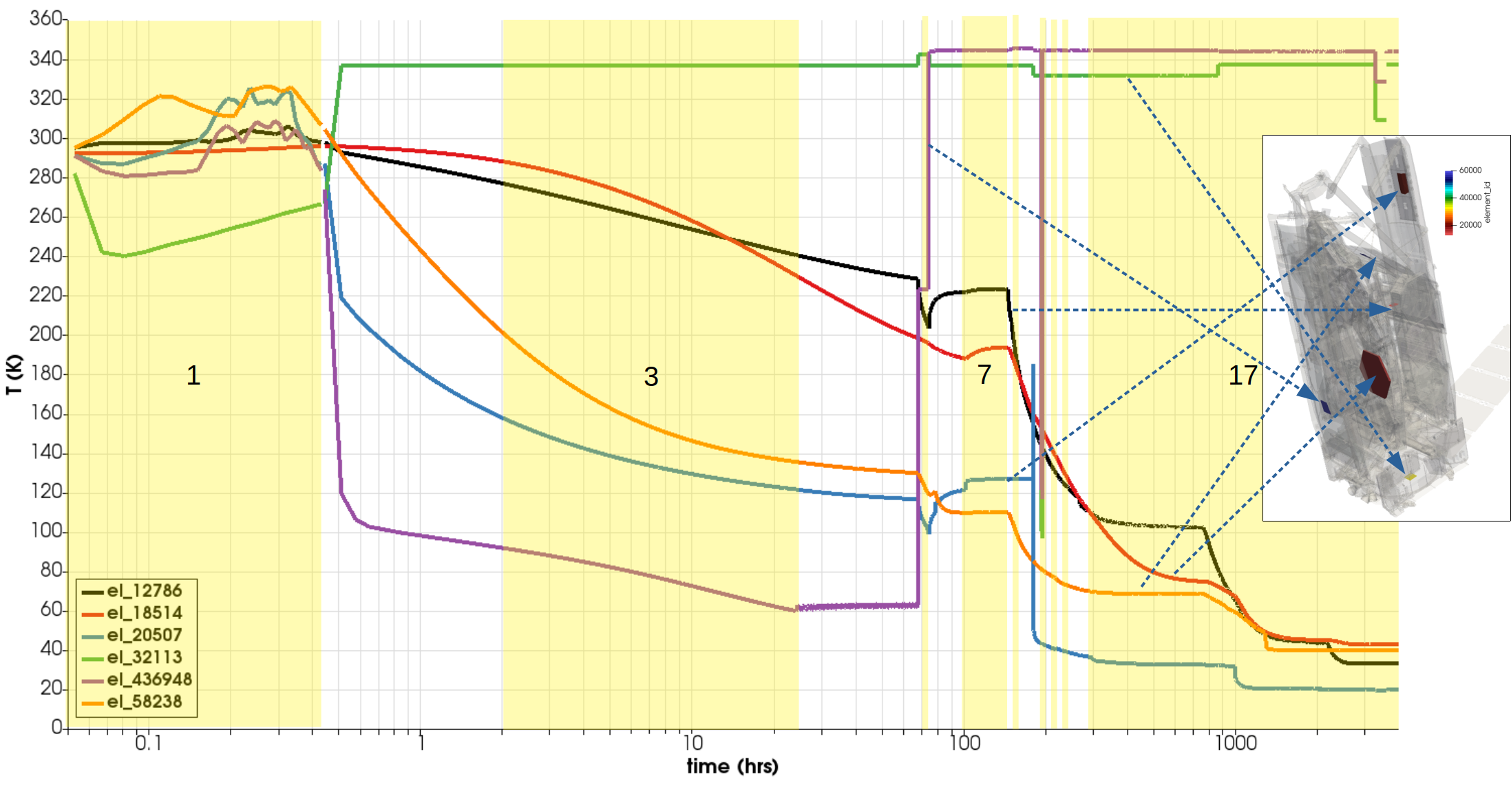
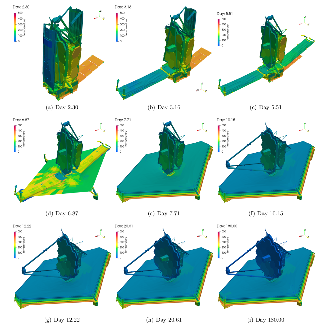
Another challenge involved capturing the time varying temperature change. Here we were provided over 13 Gb of binary data in the SINDA format. These files specified the temperatures for all TSS thermal “nodes” at up to sub minute intervals over the 180 day period of interest. This required writing another parser. Figure 2 illustrates how temperature changes on several components of interest (inset). We can see that while most components are generally cooling, there are some surfaces that undergo a warmup. This includes the pallets providing support for the sunshade. They are originally folded up, and mostly shaded by the bus. Their deployment starting at day 3 brings them into sun view and hence any water that may have collected on them is expected to flash off.
The next challenge involved coming up with some scheme for obtaining contaminant deposition over the 180 day period of interest. Despite our best efforts over the years to speed up CTSP as much as possible, the code runs at sub real time speeds. The reason is that typical molecules move around at several hundred meters per second. Resolving their individual motion on spatial scales of a satellite requires integration time steps near a microsecond. Hence, around 1 million time steps are needed just to simulate one second of real time. Regardless of how much optimization one can do, simulating 1 million steps in a single second is beyond current computational capabilities. But even that is not enough. A simulation running at real time would require 180 days of run time. There are not many project managers willing to tolerate such a long delay to a solution! As such, we devised a method where the 180 day period was divided into 200 individual time points. The spacing between them was not uniform, with more points stacked towards the front when outgassing rates and temperatures were changing more rapidly. We used each time point to compute a steady-state deposition rate at that time. This rate was then integrated forward (just using the first-order Forward Euler method) to update the amount of contaminants on each surface until the next time point. The input files were generated using a Python script, and took advantage of newly developed support for utilizing variables and breaking up the inputs among multiple files.
While this approach was fairly straightforward for integration through the same geometrical configuration, it introduced some challenges between stage transitions. This transition was captured by outputting the amount of adhered material on each surface element according to its TSS submodel and id. The simulation was then restarted using the next geometry file. During loading, the data from the restart file was loaded onto the new geometry. Mass conservation required that every surface element of the old model mapped to a surface element in the new file. While this was mostly the case, there were some instances where this mapping was incomplete. For example, the sunshield membrane is initially protected by covers. These covers are removed after stage 7, and the resulting rolls end up on the spacecraft (warm) side of the pallets. The TSS model did not include these rolls until stage 10 so we had to incorporate them into the earlier stages. Furthermore, as one may expect, there is no element node correspondence between the covers and the rolls. We ended up specifying a range of elements id (for the membrane) that had all their mass uniformly redistributed to a different set of element ids (for the rolls). Similar approach was used to model the tensioning of the sunshield. The sunshield was modeled using just a single double-sided surface in stage 9, but it turns into 5 double-sided surfaces in stage 10. This wouldn’t be too bad if the geometries matched as we could just use the data from the single sided model for the two outermost layers in the tensioned configuration. Unfortunately, the node ids here did not agree at all. We were forced once again to redistribute the stored mass utilizing a range of ids. While this helped us preserve mass conservation, it led to a loss of data locality during this phase. Luckily it turns out that not much mass deposited during this phase.
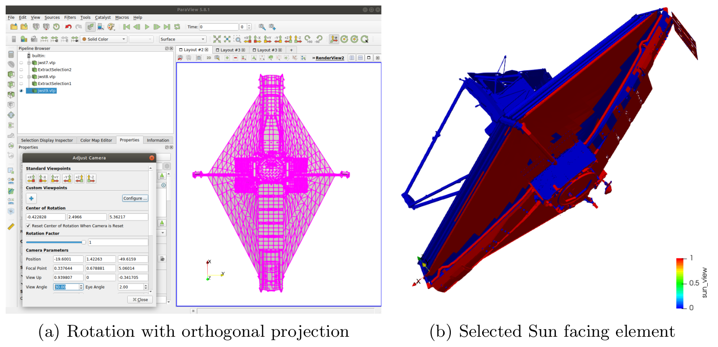
A yet another required input involved flagging surface elements with a direct line of sight to the sun. This data was needed since we assumed that 10% of molecular contaminant impacting a surface exposed to sunlight permanently attaches due to process called photopolymerization. This chemical binding makes it possible for contaminants to stick to surfaces that are otherwise too warm to act as collectors. We set these elements with the help of Paraview. Each of the 17 geometry models was rotated to align the solar panel with the screen, and then, using the orthogonal 2D projection, we simply selected and exported all visible elements. Figure 3 visualizes the sun-facing elements for the final deployed configuration.
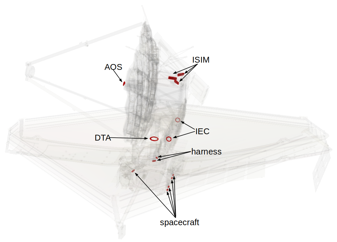
At this point, “all” that remained was setting material sources and surface deposition behavior. There were two types of sources to consider: vents and surface outgassing. The vents captured outgassing from internal components that were not part of our model. For example, none of the electronics boxes making up the guts of the spacecraft or the Integrated Science Instrument Module (ISIM, the big structure behind the primary mirror) were included in the geometry files. We were provided a time-dependent mass flow rates based estimated based on the total amount of mass present within each vented volume. The vent locations are shown in Figure 4. We also had to specify the outgassing rates. Here we utilized material testing information provided to us from the spacecraft vendor Northrop Grumman which we combined with some limiters and correction factors to avoid non-physical mass production at high temperatures.
Finally, having material sources, we also had to specify surface impact behavior. The fairly standard approach of using temperature dependent sticking coefficient was used for molecular contaminants. The actual temperature variation was derived from a QCM thermogravimetric analysis (TGA) of general spacecraft outgassed materials. A different model was used for water. Here we used a paper of Murphy and Koop to computer the saturation vapor pressure of water at surface temperature. This vapor pressure can be used to compute the maximum mass flux out of surface, assuming infinitely large reservoir (i.e. what you would have above a lake). Then utilizing the surface area and the integration time step we can calculate the number of molecules leaving the surface. This value is next compared against the actual number of molecules actually stuck to the surface. The smaller value gave us a desorption “capacity”. Water molecules impacting the surface were reflected until the capacity got depleted, after which they would completely stick. This saturation vapor pressure was also used to desorb water on each stage start up. This allowed us to model sublimation of ice that previously collected on a cold surface but subsequently warmed up, such as after the lowering of the sunshield support pallets. The paper goes into much detail of this process so please refer to it for more information.
Results
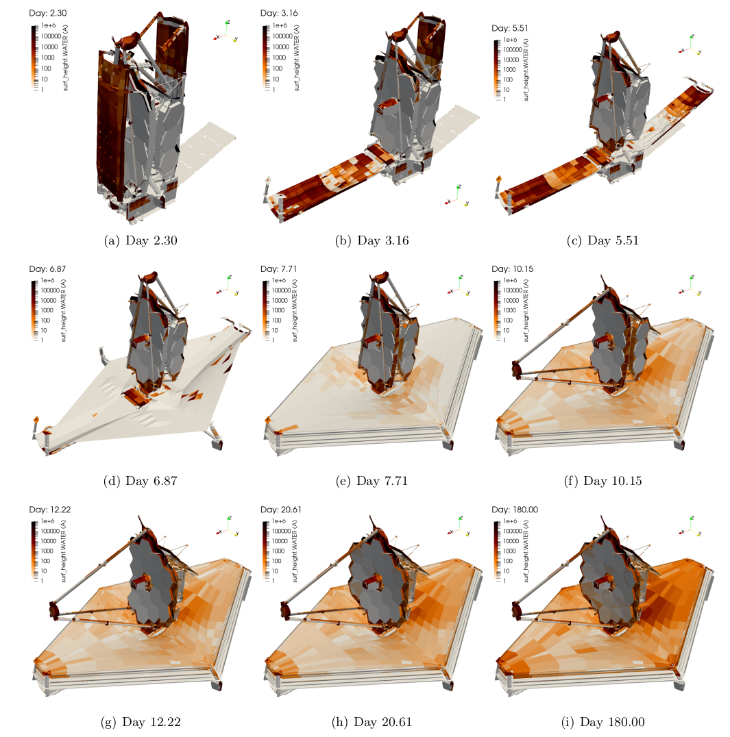
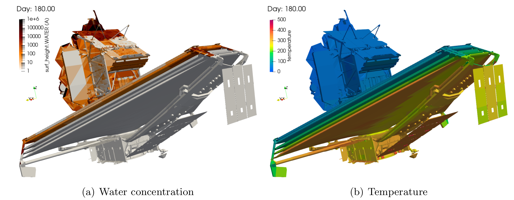
After all the effort that went into setting up the simulation, getting results was almost anticlimactic. Figure 5 shows the predicted water ice deposition thickness during the first 180 days post launch. Figure 6 shows the corresponding temperature variation. It is important to note that initially water collects on the pallet membrane covers. However the cover is rolled away around day 4, leaving behind a pristine sunshield. The ice that subsequently accumulates was within the allowable limits for the thermal design. Similarly while we observe some icing on the primary mirror, the levels were well within tolerance.
In Figure 7 we plot the ice thickness on the sun-facing spacecraft side. As expected, nothing sticks here.
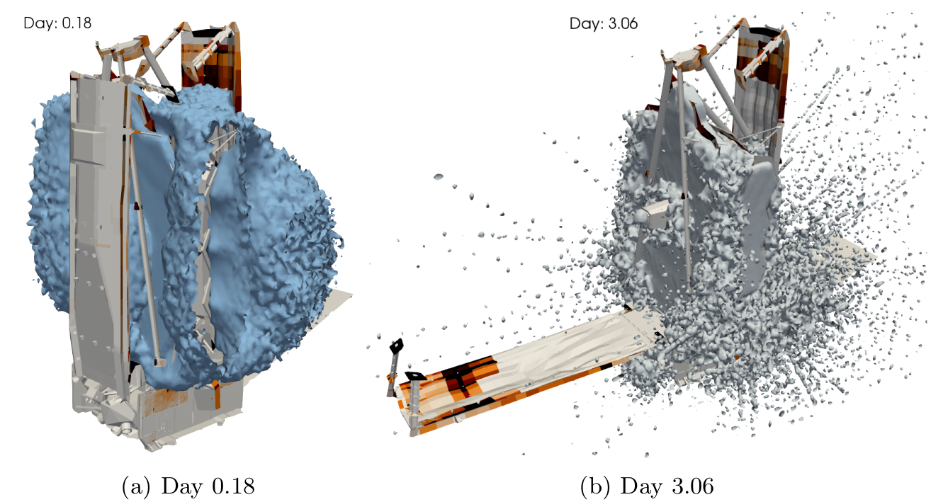
The work presented here was actually a follow up to a 2012 contamination analysis performed at NG using the design at the time. That analysis considered just three deployment configurations and was also run using ray traced radiation heat transfer view factors. The use of thermal codes for contamination analysis is quite common, since in the absence of collisions and ionization, molecules move in straight lines just like photons. The downside of this approach is that ray tracing does not produce any intermediate information about molecular concentration between surfaces. CTSP on the other hand advances the entire representative gas population together through small integration time steps. Since molecules “exist” between surfaces, we can scatter their positions to a volumetric grid to visualize the number density variation. This is shown in Figure 8. Here we see the regions with high water number density. These plots help us observe the major sources of water, and also obtain an insight into how the molecules mover around. Initially post launch, the majority of water is originating from the folded up sunshield, ISIM, and the primary mirror. Due to the closed up “cocoon” this water takes some time to get out. Later by day 3, the observatory is more opened up, making it easier for the water to get out. By now, the surface outgassing rate has also reduced, and in fact observatory vents are becoming more relevant.
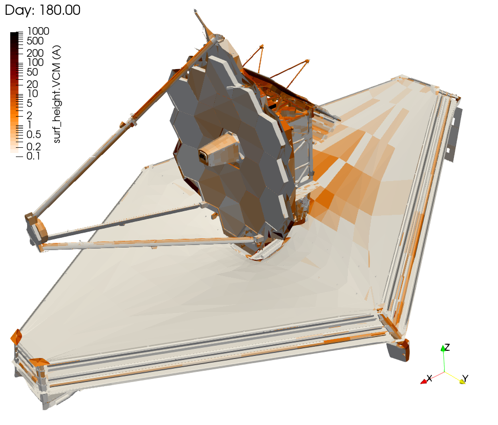
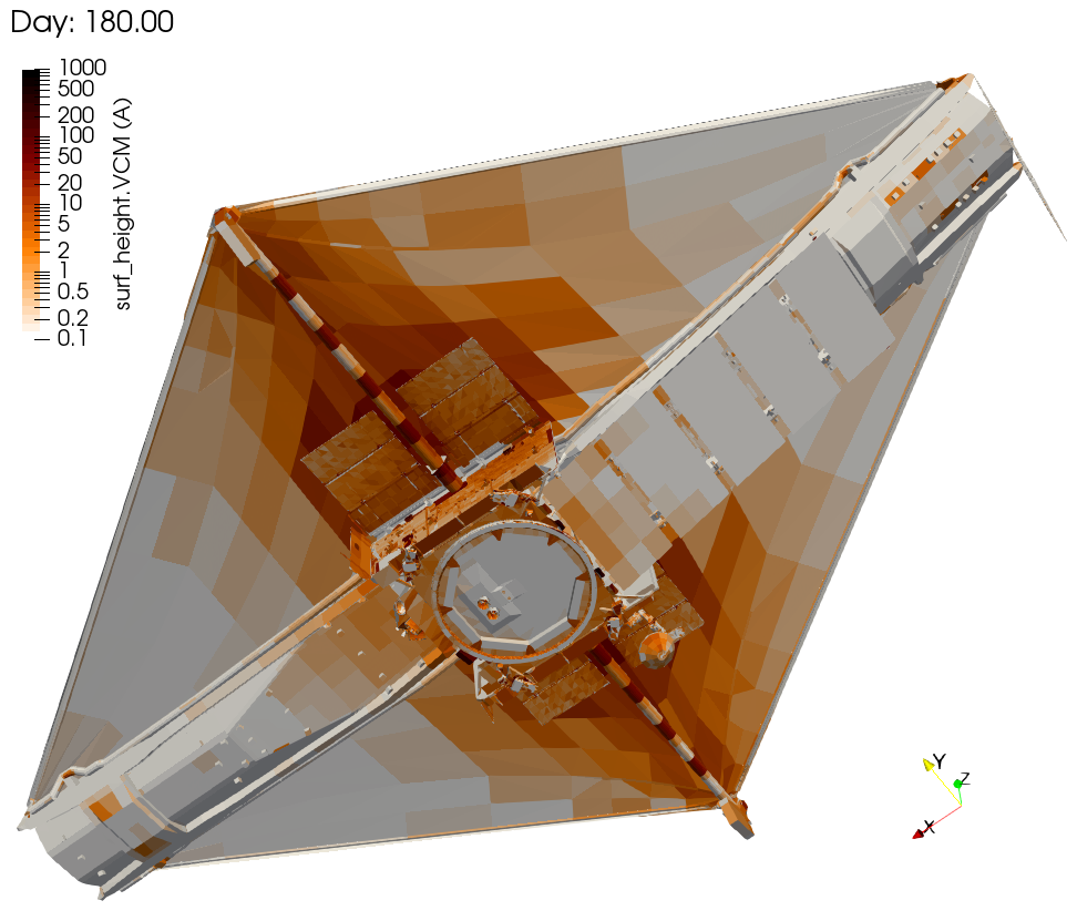
Finally, Figure 9 visualizes the molecular contaminant deposition. What is interesting to note here is that in the case of VCM, we do observe deposition even on the warm sun-facing side. This is due to the photopolymerization effect. The predicted levels were also within the allowable limits. Still, I must admit that I was very happy that nobody from NASA called me during the commissioning phase. When it comes to contamination, no news is good news. And as we have all seen by now, the telescope continues to stun with every new image.