Detailed Surface Model

PIC-C recently developed a new model for treating the vacuum-surface interface. This model will be presented at the 34^th International Electric Propulsion Conference (IEPC 2015) in Kobe, Japan. If you happen to be attending, please stop by! Link to the paper will be posted after the conference.

Residence Time

In the rarefied gas / contamination / radiation transport communities it is customary to define a sticking coefficient that determines whether a molecule is reflected upon impacting a surface. However, this is just a simplification. In reality, an impacting molecule temporarily attaches to the surface until, due to various random processes, it gains enough energy to leave. The time spent on the surface is known as residence time [1],
$$\tau_r = \tau_0\exp(E_a/RT)$$

This new model computes the residence time for impacting molecules, and if it’s greater than the simulation time step (Delta t), the molecules are adsorbed into a surface layer. In addition, our model allows objects to consist of a base substrate containing multiple trapped gases. These gases slowly diffuse into the surface according to
$$\frac{dm}{dt}=Cm\frac{\exp(E_a/RT)}{\sqrt{t}}$$

A separate desorption algorithm computes the rate of molecules leaving the surface layer for the bulk gas phase according to first-order desorption (valid if surface layer thickness is less than a monolayer),
$$\frac{dN}{dt}=\frac{1}{\tau_r}N$$

Contamination Transport Simulation Program (CTSP)

This algorithm is implemented in our Contamination Transport Simulation Program (CTSP). CTSP is a 3D particle code, similar to DSMC or PIC, but with the exception that it does not use a volume mesh for the particle push. Such a mesh is used in the PIC method to compute electrostatic forces, and by DSMC to group particles for collisions. Instead, the code uses point-cloud data to specify background force, and an inverse distance weighting method to collect forces at the particle location. An octree is used to store the surface elements and the point cloud data, if any.

Examples

Temporal Effects

Besides being based on physical parameters, this new surface model also allows us to resolve temporal effects. We often observe pressure spikes during thermal vacuum testing. In vacuum, water condenses around -100^oC (the actual temperature for any gas can be obtained from vapor pressure graphs, or for water, the Arden Buck equation). If a surface warms up and goes through this temperature, all water that was adsorbed will flash off, resulting in a pressure spike. The new surface model captures this behavior automatically. This is in fact demonstrated in the video in Figure 1. In this animation, a thruster is operating in a chamber equipped with a beam dump. The beam dump is initially sufficiently cold to condense the propellant. Later, gas is injected into the chamber through a port. This could be part of an experimental setup to characterize the impact of background pressure on the thruster operation. Next, the beam dump is allowed to warm up. This is implemented in the code by linearly increasing the object temperature. As the temperature crosses the condensation temperature, the condensed propellant flashes off in a pretty impressive cloud that soon fills the entire chamber.

Shroud Temperature

This surface model also allows us to resolve the “sticking coefficient” naturally. For surfaces above materials’ condensation temperature, the residence time will be very short so the molecules will not stick. We can demonstrate this effect by comparing partial pressure of water in a chamber containing a thermal shroud. This is shown in Figure 2. The chamber contains a test article with an initial surface layer of water, and also water outgassing from the substrate. The plot on left shows the case with a 300K shroud. On right, the shroud is at 100K which is cold enough for water to stick. Besides the pressure being higher in the 300K case, we also see a higher deposition thickness on the cryopumps. This arises naturally from mass conservation. In a closed system, such as this vacuum chamber, the source rate is balanced by the sink rate,
$$\Gamma_{hw}A_{hw} = \Gamma_{sink}A_{sink}$$
With a cold shroud, \(A_{sink}=A_{shroud}+A_{scva}+A_{pump}\). With the shroud at 300K, the sink area reduces to \(A_{sink}=A_{scav}+A_{pump}\). Since \(A_{shroud}\gg (A_{pump}+A_{scav})\), the pump flux is greatly increased.

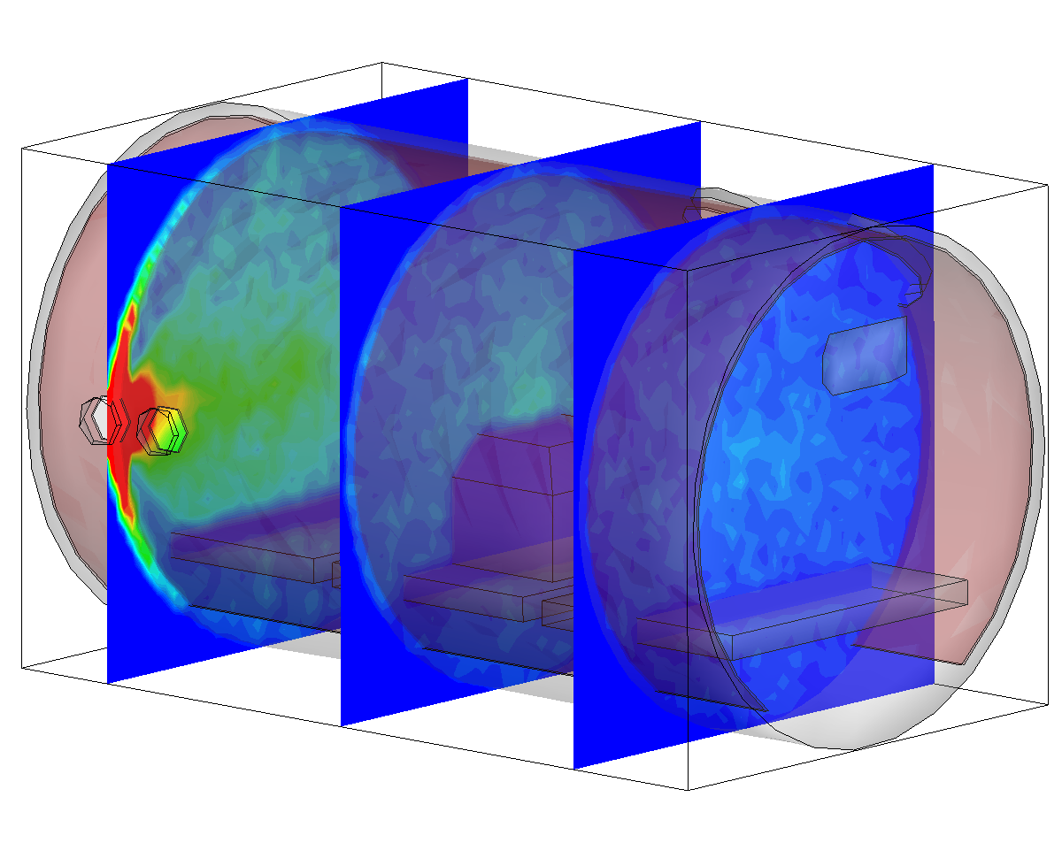
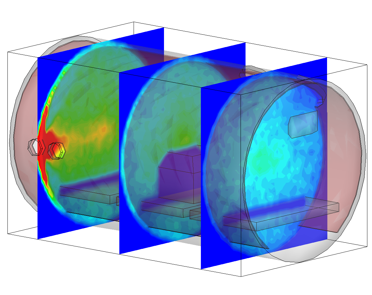
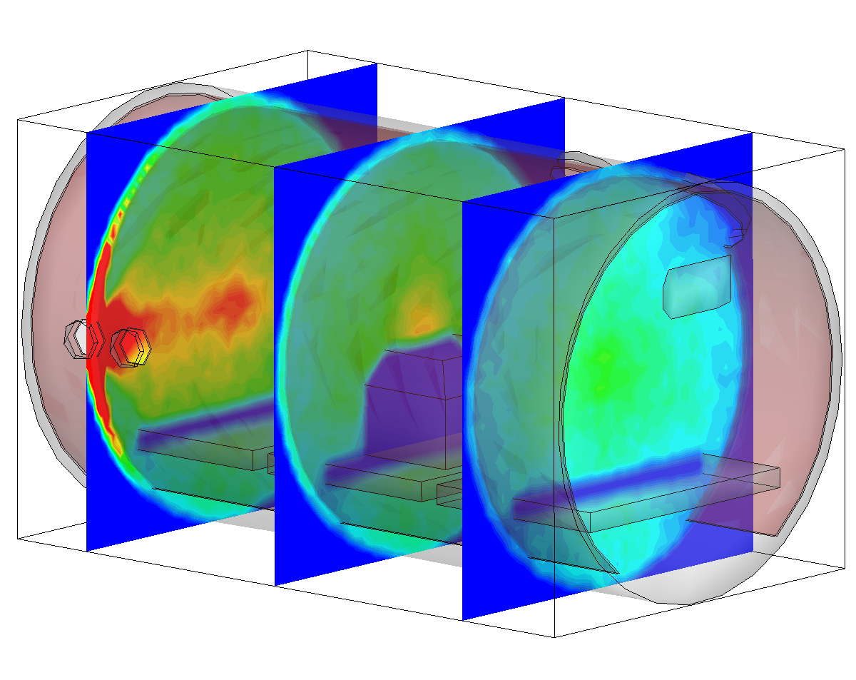
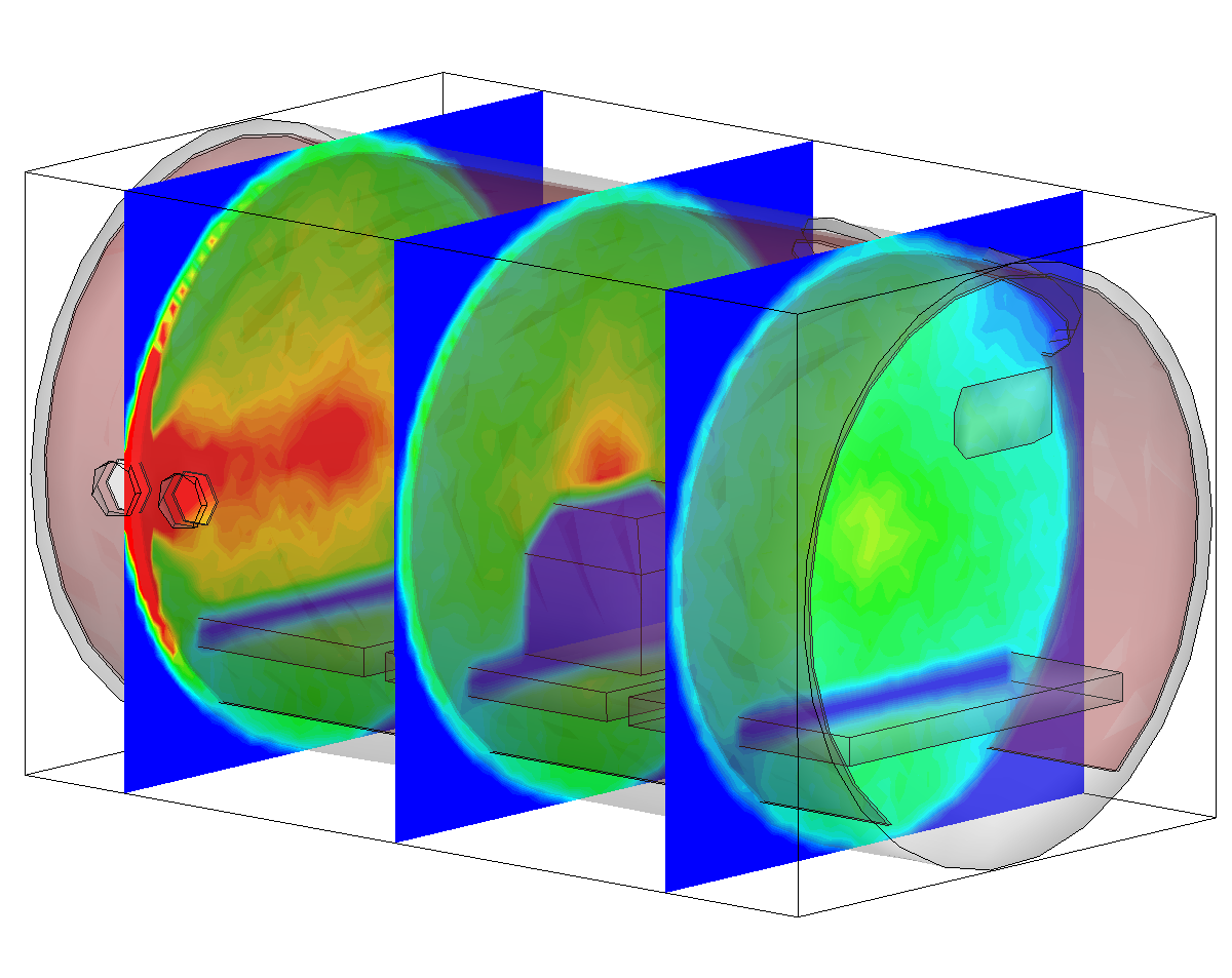
By using different activation energies for different materials, we can obtain the spatial distribution of that population. This is shown in Figure 3. In this simulation, the test article was assumed to consist of trapped nitrogen and water. The small “electronics box” was assumed to be at a hotter temperature, and also an outgassing source of some hydrocarbon. The shroud was cold enough to condense water (and the hydrocarbon) but not the nitrogen. We can see that the nitrogen density is more uniform than that of water, but there is still a spatial non-uniformity below the platens. However, if the simulation was run long enough to deplete vast majority of the trapped nitrogen outgassing from the test article, we would see the nitrogen distribution to equalize.

Finally, the last set of pictures shows snapshots from another run which considered gas injection in to a chamber. This could correspond to a gas leak, or early phases of a chamber repress. We can note that the pressure is again non-uniform. Also, due to thermal effects and the geometric configuration of the port and the cutout in the shroud, some molecules impact the back side of the shroud and become trapped in the narrow region between the shroud and the wall. After a sufficiently long time, these molecules will bounce out of the gap and find their way to the pump.

Conclusion

This article presented results from a newly developed model for the vacuum/surface interface based on activation energies. The model allows incoming molecules to adsorb to a surface layer. The materials can also contain trapped gases slowly diffusing to the surface. Desorption model is used to inject molecules from the surface layer into the gas phase.

Please contact us if you are interested in obtaining a copy of the software. Also please let me know if the videos do not work for you – I am still new to HTML5 video and not sure which codes have the widest support.

References:
[1] Tribble, A., Fundamentals of Contamination Control , SPIE, 2000