Spacecraft Surface Charging

When modeling plasmas, we are often dealing with charged particles interacting with a solid surface. This results in a net current flow into said surface. How this current is treated can have a profound effect on the results of a given simulation – do we treat the surface as a grounded conductor and ignore the current? Do we treat it as a perfect insulator and charge the local area of the surface? Or, do we conduct the current through the surface based on the real conductivity and layout that we are attempting to model?
So let’s say you have a spacecraft that is about to encounter some charged particles. What is the best way to handle it?
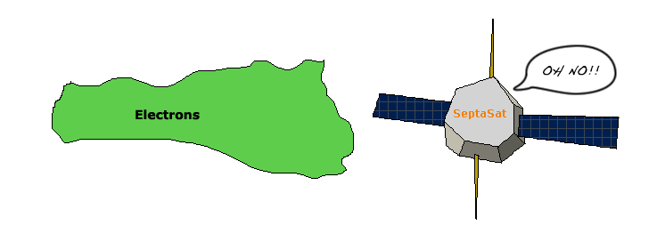
Figure 1. The problem – how do we deal with charged particles hitting a surface?
Note: This tutorial assumes you are already familiar with surface meshes and general plasma modeling practices. For a refresher, see the PIC tutorial.
Grounded Conductor
 The first approach is the easiest, and by far the most common. When a charged particle hits a surface, simply throw it away. The physical assumption being made here, is that the surface in question is a uniform conducting body that is well grounded such that any net charge will be instantly zeroed out by the ground. This is often not true in space applications since spacecraft have no real ground other than the bus itself. This approach can also not handle any sort of non-conductive elements (solar arrays, dieletrics, etc). This can be a good assumption for a laboratory setup, however.
Perfect Insulator
If we want to actually charge a surface, the basic charging equation is very simple on its face:
$$\phi=\frac{q}{C}$$
where \(q\) and \(\phi\) are charge stored on the surface and the potential of the surface (what we are after.) The hard part is the capacitance, \(C\).
The second approach we will look at for charging calculations is to detect which surface element a particle hits and simply apply that particle’s charge to that element. The assumption being made here is that the surface is a perfect insulator – the charge stays in the exact place it impacted the surface and is never carried away. Similarly, one surface element has no knowledge of the charge state of it’s neighbors. This sort of approximation is not bad for insulators, but would be totally invalid for a material with even a small amount of conductivity. Indeed, very few space materials are TOTALLY non conductive – in many cases materials are carbonized to allow for charge to dissipate slowly over time (we wouldn’t want any ESD events!)
If one is to take this approach, then we can treat each element as a totally isolated, non conductive blob with a current hitting one end – basically this is your run of the mill parallel plate capacitor. We can therefore model the charge buildup on the element as: \(C=\epsilon\dfrac{A}{dz}\) where \(\epsilon\) is the permittivity of the material, \(A\) is the area of each “plate”, which in our case is just the area of the element, and \(dz\) is the distance between the “plates”, or the thickness of the element.
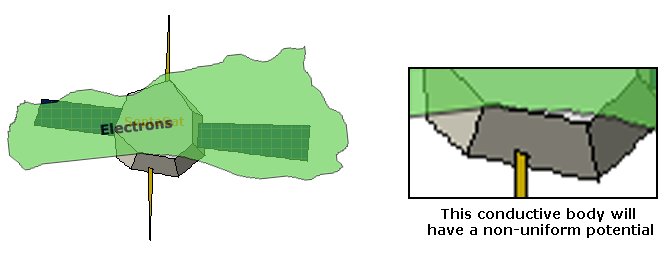
Figure 3. The conductive body is not uniformly charged.
Component Based Charging
One easy way to compromise between these two methods is to separate an object into sub-components that be either conductive or non-conductive. This way, metals will not accumulate charge, and dielectrics will. The fact remains, however, that most materials will dissipate over time, and that conductors without a good ground will charge up (albeit in a uniform fashion) over time.
To deal with the conductors charging over time, conductive components can really be treated much as we did the dielectric elements – as a single charging body (or more useful, to say that each set of electrically connected components is an individual body.) For example, long booms may be conductive, but not electrically connected to the spacecraft BUS.
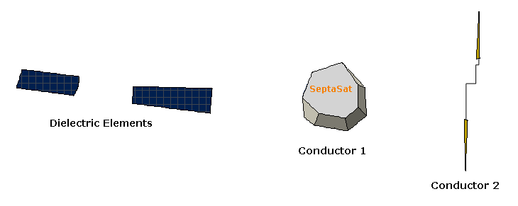
Figure 4. The object is split into two conductor groups and one dielectric group.
The primary difference between this case and the pure dielectric case is that we cannot approximate the capacitance as a simple parallel plate based on a characteristic length. Calculating the capacitance of a complex conductive body is by no means a trivial task and it is not going to be discussed here. One commonly used cheater method is to simply treat it as a sphere of roughly the same size (radius \(r\)), in which case the capacitance can be approximated as \(4\pi\varepsilon r\)
Then the overall charging equation becomes:
$$\phi=\frac{q}{4\pi\varepsilon r}$$
This will get us to a point where we have a reasonable approximation of the charge state over time, except for the one remaining problem of the static dissipative materials. To really solve this problem we have to follow the current and see where it goes. This is not nearly as daunting as it may seem, however.
Charge Propagation
Let’s first make the assumption that we are talking about small levels of conductivity (< 1e-7 mho or so). In this regime, one element can see its neighbors, but that is about it. So all we really need to do is loop through all the elements and see what the balance is between each element and it’s local neighbors – the local electric field. Solving the local electric field is trivial once we have the potential map of the surface:
$$\vec{E} = -\nabla \phi$$
Now that we have the electric field, and we know that elements see their neighbors, let’s think about what we really mean by “neighbors”. Of course this includes the elements right next door on the surface, but charge also flows into the surface. Beneath a surface, there is typically a conductor at some point so we will often have each element have a link to each of it’s neighboring elements as well as a conductive body underneath.
So now that we have the electric field mapped out, we know how charge moves over the surface, all we have to do is move it. First we get a current density, \(j\) based on the electric field, and the conductivity, \(\sigma\): \(j=E\sigma\)
Then we convert the current density to a current based on the cross sectional area of the element:
$$i=jdydz$$
With a current, all we do is multiply by time to get the amount of charge moved – simple right?
Actually, this is where we get into trouble. Every little bit of charge that is moved changes the overall map of the electric field. For this reason, a very small timestep must be used to ensure that our field measurement is still valid. With many plasma modeling codes, a constant timestep is used since the bulk plasma parameters do not significantly change. In this case, however, the charge state, and local electric field, can vary substantially over time so a dynamic timestep must be used. A guideline that generally works is to never remove more than 1% of an element’s total charge in one timestep. This can be pushed a bit if you are feeling gutsy, but if you move too much charge at once, you will end up with a potential map that looks “lumpy” instead of a nice uniform gradient. In the extreme case, you can even get two elements that oscillate between positive and negative as they swap charge back and forth. Since a constant timestep must be used by all elements, the simplest thing to do is to base your timestep on the element pair with the greatest electric field (ie the smallest timestep.) The timestep can then be calculated as
$$dt=0.01\left|\frac{q}{i}\right|$$
and then we just move the charge around based on the current \(dq=idt\)

Figure 5. With too large a timestep, charging becomes non-uniform.
Example – a Semiconductive “Wire”

Figure 6. Semiconductive strip example.
As an example, let’s examine a simple 1D strip of elements with a constant flux at one end and a ground plane at the other end. This example is coded up in the Matlab script, charge1d.m. Running the example with the default parameters, we see that the strip will reach a steady state with a potential linearly decreasing from 1067V at the input end, to 0 at the ground plane. As a check, we can imagine that this strip is simply a wire with a current flowing through it equal to the input flux. We can calculate the
resistance of the wire as:
$$R=\frac{L}{\sigma A}$$
Assuming that our current is simply the flux (times cross sectional area and electron charge of course), this leads to a trivial calculation of the potential drop using Ohm’s Law:
$$ V=IR$$
This gives us an analytical answer of 1068V, pretty close to our simulated 1067!
Try playing with the conductivity of the material to see how much conductivity is required to maintain given potentials. You can also try forcing a bias potential and see how the strip will float based on that potential.
This code can be expanded into a 2D, or 3D simulation fairly easily. The only real modification would be to have more inter-element connections. In these cases, however, even more attention must be paid to the speed at which charge is being removed from an element – if an element conducts charge to 5 different locations (say 4 neighbors plus an underlying conductor) then all of those paths have to be taken into account when deciding on the timestep to ensure that after we move charge to one element there is still some left
to move to the others.
References:
1. Barrie, A. Modeling Differential Charging of Composite Spacecraft Bodies Using the Coliseum Framework, Masters Thesis, Department of Aerospace and Ocean Engineering, Virginia Tech, 2006.
2. Barrie, A. Modeling Surface Charging with DRACO Electric Propulsion Simulation Package. Joint Propulsion Conference and Exhibit, 2006.