Leapfrog Particle Push (Velocity Integration)

In this article we’ll discuss how to integrate particle velocities in kinetic plasma simulations. This particle push is an extremely important part of the simulation process. It’s basically the engine that drives these codes. It results in the simulation macroparticles advancing to new positions in response to the forces acting on them. Our previous article on the particle in cell method briefly introduced this concept as well as the leapfrog method used to perform the integration. Here we expand on this topic.
First, let’s take a look at the governing equations. They are simply the definition of velocity
$$\displaystyle \frac{d\vec{x}}{dt} = \vec{v}$$
and acceleration
$$\displaystyle \frac{d\vec{v}}{dt} = \frac{q}{m}\left(\vec{E}+\vec{v}\times\vec{B}\right)$$
This second equation is basically Newton’s Second Law, with the force being the Lorentz Force. Of course, additional forces, such as gravitational, centripetal, and magnetic pressure force may also be present. Whether these are to be included will depend on the details of your problem, and the relative magnitude of the forces. However, generally the Lorentz force dominates, and the remaining forces are neglected. Our goal is to integrate this system in time.
v x B = 0 case
We will start by looking at the case where the second term in the Lorentz force drops out. This implies that either there is no magnetic field, or the particle motion is in direction parallel to the magnetic field line. We will discuss how to push particles in presence of magnetic field (v x B rotation) in the second part of this article. Here we have
$$\displaystyle \frac{d\vec{v}}{dt} = \frac{q}{m}\vec{E}$$
Forward Difference Scheme
Integration of this equation appears to be trivial. We could take the velocity at some time “n” and use it to move the particle by a finite distance.
$$\displaystyle\frac{d\vec{v}}{dt}\sim\frac{v^{n+1}-v^n}{\Delta t}=\dfrac{q}{m}\vec{E}$$
$$\displaystyle\frac{d\vec{x}}{dt}\sim\frac{x^{n+1}-x^n}{\Delta t}=v^n$$
and implement it as (Equation 1):
/*grab electric field at current position*/
E[0]=EvalE0(x[0]); E[1]=EvalE1(x[1]);
/*get new velocity at n+1*/
v2[0] = v[0] + q/m*E[0]*dt;
v2[1] = v[1] + q/m*E[1]*dt;
/*update position*/
x2[0] = x[0] + v[0]*dt;
x2[1] = x[1] + v[1]*dt;
/*copy n+1 velocity to n*/
v[0]=v2[0];
v[1]=v2[1];
This solution is simple, but unfortunately, incorrect. To see why, let’s look at an even simpler example: a one dimensional oscillator around x. In plasma physics, such a solution could correspond to an electron oscillating around a stationary ion at the fundamental plasma frequency. Position, as a function of time, is given by \(x=\cos(\omega_p t)\). The analytical solution for velocity and acceleration is, \(v=-\omega_p\sin(\omega t)\) and \(a=-\omega_p^2\cos(\omega t)=-\omega_p^2x\), respectively. We have an expression for acceleration. We want to integrate it, numerically, and retrieve the original expression. As a little aside, from the acceleration expression we see that the electric field for an oscillating particle is \(E=-(m/q)\omega_p^2x\).


Figure 1. Oscillator results obtained with the simple forward difference scheme.
The forward difference method is implemented in the attached Excel spreadsheet. Excel can be quite handy for algorithm prototyping if you don’t have access to tools such as Matlab or it’s free clone, Octave. However, be careful of a bug in the Excel equation evaluator. Excel does not use correct operator precedence with powers, and -5^2 evaluates to 25, instead the correct -25. Such expressions need to be written as -(5^2).
Solution is plotted below in Figures 1a) and 1b). The first curve shows position versus time. The theoretical curve is shown in blue. We can see that the particle indeed oscillates between 1 and -1. What’s important is to note that the magnitude of the wave does not change over time. This is definitely not the case with the numerically obtained red dashed curve! Although the system is oscillating at the original frequency, the amplitude keeps increasing. This means that the particle is getting farther and farther from the center. In other words, the particle is gaining energy. But this is completely non-physical; this energy increase is purely numerical. Figure 1b) shows the same result on a velocity/position phase plot. Phase plots like these can often give us additional insight into the problem beyond the standard position vs time plots. In this case, the correct solution is an ellipse with the axis parallel to the coordinate system. Clearly, it should not be a spiral, as is the case for the numerical scheme.
What’s interesting is that this scheme will not give the correct result despite of how small a time step you use. Try it.
Error Analysis
We can prove this analytically. The standard approach is to assume that the solution varies from one time step to another by a linear amplification factor g. We can then write
$$\begin{array}{rcl}
x^{n+1} &=& gx^n \\
x^n &=& gx^0\\
v^n &=& gv^0
\end{array}
$$
For stability, we want the magnitude of g to be less than or equal to 1. Otherwise the value of x will continue to grow and the solution will not converge. To solve for g, we rewrite Equation 1 in a matrix form as
$$
\left[\begin{array}{cc}
g-1 & \omega_p^2\Delta t\\
-\Delta t & g-1\end{array}\right]
\left(\begin{array}{c}
v_0\\x_0\end{array}\right) =
\left(\begin{array}{c}
0\\0\end{array}\right)
$$
One solution is the trivial solution, x=0 and v=0. But that’s not of much interest. Instead, we want to compute the null space (or kernel). You can check for yourself that this is analogous to solving for zero determinant, \((g-1)^2+\omega_p^2\Delta t^2=0\), or \(g=1\pm i \omega_p \Delta t\). The magnitude, \(\left|g\right|^2>1\) regardless of how small a time step is selected. Hence, the upward difference method is inherently unstable.
Leapfrog Method
The problem with the Forward Difference method arises from the fact that it uses velocity at time “n” to push the particle from “n” to “n+1”. What makes more physical sense is to use the average velocity, the velocity that would exist at time “n+1/2”. This is the premise of the leapfrog method. Velocity and position integration leap over each other, being displaced by half a time step. This is illustrated in Figure 2 below (this same figure was used in the article on the particle in cell method). In our implementation, particle positions exist at the integral time steps, while velocity exists at the half times. This introduces little difficulty into particle loading, since source sampling will result in velocity and position at the same time step. The usual method is integrate the velocity (but not position) of all newly loaded particles backwards through -0.5dt. The implementation then follows:
/*sample new particle*/
[x,v] = SampleParticle();
/*move velocity back by 0.5dt*/
E = EvalE(x);
v = v - 0.5*q/m*E*dt;
/*main loop*/
/*update velocity and position*/
E = EvalE(x);
v = v + q/m*E*dt;
x = x + v*dt;
Implementation of this method is shown in Figure 3. This time, the analytical expression is restored.
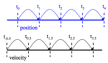
Figure 2. Schematic of the leapfrog method. Position is evaluated at integral time steps, while velocity is evaluated at half times.


Figure 3. Oscillator results obtained with the leapfrog scheme.
We can compute the stability condition for the Leapfrog method using error analysis similar to what was done for the Forward method.
$$
\left[\begin{array}{cc}
g^{1/2}-g^{-1/2} & w_p^2\Delta t\\
-g^{1/2}\Delta t & g-1\end{array}\right]
\left(\begin{array}{c}
v_0\\x_0\end{array}\right) =
\left(\begin{array}{c}
0\\0\end{array}\right)
$$
The characteristic equation obtained by setting the determinant to zero is \(g^2 – (2-\omega_p^2\Delta^2t)g+1=0\). Using the quadratic formula, we obtain the solution to be
$$
\begin{array}{rcl}
g &=& \dfrac{\left(2-\omega_p^2\Delta^2t\right) \pm \sqrt {\left(2-\omega_p^2\Delta^2t\right)^2-4}}{2}\\
&=& 1 – \dfrac{\omega_p^2\Delta^2t}{2} \pm \sqrt{\dfrac{\omega_p^4\Delta^4t}{4}-\omega_p^2\Delta^2t}\\
&=& 1 – \dfrac{\omega_p^2\Delta^2t}{2} \pm \omega_p\Delta t\sqrt{\dfrac{\omega_p^2\Delta^2t}{4}-1}
\end{array}
$$
The system is stable only if the expression under the square root is less than 0. Then \(g = 1 – \dfrac{\omega_p^2\Delta^2t}{2} \pm i \omega_p\Delta t\sqrt{1-\dfrac{\omega_p^2\Delta^2t}{4}}\). Magnitude of this complex number is given by the complex conjugate, which in this case equals to 1. The system is therefore stable and neutral. In terms of the time step required, we obtain that for the Leapfrog Method, \(\Delta t < 2/\omega_p\). Don't forget to take a look at Part 2 for full implementation of particle push, including E and B fields.
Attachments:
integration.xlsx (numerical integration the harmonic oscillator)
References:
Toshiki Tajima, Computational Plasma Physics, Westview Press, 2004.
I don’t understand about the idea of linear amplification factor g. The positions and velocities are real number, so Why can g be a complex number? And does g depend on n?