Finite Element Experiments in MATLAB

This guest article was submitted by John Coady (bio below). Would you like to submit an article? If so, please see the submission guidelines. If your article is on scientific computing, plasma modeling, or basic plasma / rarefied gas research, we are interested!
In my previous post I talked about a MATLAB implementation of the Finite Element Method and gave a few examples of it solving to Poisson and Laplace equations in 2D. The examples that I provided all used piecewise linear polynomials in the Finite Element algorithm. This time I will show how the accuracy can be improved by using higher order polynomials and conduct a number of experiments to show the improvement in the results.
We will be using Finite Element Method to solve Laplace and Poisson equations of the following form.
$$ -\nabla \cdot (k(x,y) \nabla u(x,y)) = f(x,y)$$
The Finite Element method converts this continuous equation to a discrete equation of the form
$$ KU = F$$
where lower case values like u(x,y) are continuous and upper case values like U are discrete. In the discrete Poisson equation, K is the stiffness matrix of size NxN, F is the load vector of size Nx1 and U is an Nx1 vector where N is the number of nodes in the mesh. With the Finite Element method the computer will assemble the stiffness matrix K and the load vector F as well as solve the equation KU=F to determine the best approximation to U.
The Finite Element method does this conversion from continuous to discrete by choosing a finite number of test and trial functions that are simple polynomials and approximating the exact solution by a combination of those polynomial functions. We will be using linear, quadratic and cubic polynomials as test and trial functions in the Finite Element algorithm to compute an approximate solution and compare the results to the exact solution.
Discretizing Poisson
One way the Finite Element method discretizes the continuous Poisson equation is as follows. Start with the continuous Poisson equation.
$$ -\nabla \cdot (k \nabla u) = f$$
Multiply both sides by a test function \(v\) and then integrate to give the weak form of Poisson’s equation.
$$ \iint (-\nabla \cdot (k \nabla u)) v\,{d}A = \iint fv\,dA$$
Next use integration by parts to move one of the derivatives off of u and puts it on the test function v.
$$ \iint k \nabla u\nabla v\,{d}A – ku’v]_{0}^1 = \iint fv\,dxdy$$
If the boundary conditions for u’ or v are zero then it is reduced to
$$ \iint ((k \nabla u))\nabla v\,{d}A = \iint fv\,dA$$
otherwise if \(u’ \neq 0\) then the term has to stay and it can be moved over to the right hand side.
$$ \iint ((k \nabla u))\nabla v\,{d}A = \iint fv\,dA + ku’v ]_0^1$$
Using the continuous Galerkin method to discritize \(u\) we get
$$ U = U_{1}\phi_{1} + U_{2}\phi_{2} + \ldots + U_{N}\phi_{N}$$
and the derivative
$$ U’ = U_{1}\phi_{1}’ + U_{2}\phi_{2}’ + \ldots + U_{N}\phi_{N}’$$
where \(\phi_{i}\) are trial functions. We next make the test function \(v\) equal to the trial function \( \phi\) and end up with.
$$ \iint ((k (U_{1}\phi_{1}’ + U_{2}\phi_{2}’ + \ldots + U_{N}\phi_{N}’))\phi_{i}’\,{d}A = \iint f\phi_{i}\,dA $$
In matrix form we get the discrete equation
$$ KU = F$$
where
$$ K = \iint k \nabla\phi \nabla\phi \,{d}A \\[0.3em]F = \iint f\phi\,dA$$
These integrals are evaluated in the finite element method using N-point gauss quadrature. The MATLAB code from the last post used linear polynomials for test and trial functions and showed how the stiffness matrix K and the load vector F are assembled and the linear system KU=F is solved to get give an estimate of U.
As we saw in the previous post, the finite element takes as input a mesh which can be generated by a tool like distmesh. The mesh contains triangular elements which are the pieces on which the polynomials are defined, a different polynomial in each triangle. The Finite Element algorithm will calculate a contribution to the large K and F matrices for each small triangle element matrix by integrating over all triangles in the mesh, one at a time.
P1 Linear Elements

As already mentioned, the polynomials are defined on each triangle in the mesh, which form a set of basis functions for the triangular element. Each basis function has a value of 1 at its node and a value of 0 at the other nodes giving it a pyramid shape over the triangle.
$$ \phi_{i} (x_{j},y_{j}) = \left\{ \begin{array}{l l} 1 & \quad \text{i = j}\\ 0 & \quad \text{i} \neq \text{j}\\ \end{array} \right.$$
In the case of linear finite elements, the basis functions are linear polynomials of degree 1 with the designation P1.
$$ \phi_{i} (x,y) = a_{i} + b_{i}x + c_{i}y$$
Each \(\phi_{i}\) has 3 unknown coefficients \(a_{i} b_{i} c_{i} \) so with three node points on the triangle element we can generate 3 equations for each \( \phi_{i} \).
$$ a_{1} + b_{1}x_{1} + c_{1}y_{1} = 1 \\ a_{1} + b_{1}x_{2} + c_{1}y_{2} = 0 \\ a_{1} + b_{1}x_{3} + c_{1}y_{3} = 0$$
or in matrix form for the first basis function,
$$ \begin{bmatrix} 1 & x_{1} & y_{1} \\[0.3em] 1 & x_{2} & y_{2} \\[0.3em] 1 & x_{3} & y_{3} \end{bmatrix} \begin{bmatrix} a_{1} \\[0.3em] b_{1} \\[0.3em] c_{1} \end{bmatrix} = \begin{bmatrix} 1 \\[0.3em] 0 \\[0.3em] 0 \end{bmatrix} $$
For all three basis functions in the triangle we get the equation of the form
$$ \begin{bmatrix} 1 & x_{1} & y_{1} \\[0.3em] 1 & x_{2} & y_{2} \\[0.3em] 1 & x_{3} & y_{3} \end{bmatrix} \begin{bmatrix} a_{1} & a_{2} & a_{3} \\[0.3em] b_{1} & b_{2} & b_{3} \\[0.3em] c_{1} & c_{3} & c_{3} \end{bmatrix} = \begin{bmatrix} 1 & 0 & 0 \\[0.3em] 0 & 1 & 0 \\[0.3em] 0 & 0 & 1 \end{bmatrix} $$
This has the form
$$ M M^{-1} = I$$
so we can determine the coefficients of the basis functions just by inverting the matrix M,
$$ M = \begin{bmatrix} 1 & x_{1} & y_{1} \\[0.3em] 1 & x_{2} & y_{2} \\[0.3em] 1 & x_{3} & y_{3} \end{bmatrix} \\[0.3em] M^{-1} = \begin{bmatrix} a_{1} & a_{2} & a_{3} \\[0.3em] b_{1} & b_{2} & b_{3} \\[0.3em] c_{1} & c_{2} & c_{3} \end{bmatrix} $$
P2 Quadratic Elements

$$ \phi_{i} (x_{j},y_{j}) = \left\{ \begin{array}{l l} 1 & \quad \text{i = j}\\ 0 & \quad \text{i} \neq \text{j}\\ \end{array} \right.$$
In the case of quadratic finite elements, the basis functions are quadratic polynomials of degree 2 with the designation P2.
$$ \phi_{i} (x,y) = a_{i} + b_{i}x + c_{i}y + d_{i}x^2 + e_{i}xy + f_{i}y^2$$
There are now 6 unknown coefficients, so we need to add 3 node points to each triangle element to generate 6 equations.
$$ \begin{bmatrix} 1 & x_{1} & y_{1} & x_{1}^2 & x_{1}y_{1} & y_{1}^2 \\[0.3em] 1 & x_{2} & y_{2} & x_{2}^2 & x_{2}y_{2} & y_{2}^2 \\[0.3em] 1 & x_{3} & y_{3} & x_{3}^2 & x_{3}y_{3} & y_{3}^2 \\[0.3em] 1 & x_{4} & y_{4} & x_{4}^2 & x_{4}y_{4} & y_{4}^2 \\[0.3em] 1 & x_{5} & y_{5} & x_{5}^2 & x_{5}y_{5} & y_{5}^2 \\[0.3em] 1 & x_{6} & y_{6} & x_{6}^2 & x_{6}y_{6} & y_{6}^2 \end{bmatrix} \begin{bmatrix} a_{1} \\[0.3em] b_{1} \\[0.3em] c_{1} \\[0.3em] d_{1} \\[0.3em] e_{1} \\[0.3em] f_{1} \end{bmatrix} = \begin{bmatrix} 1 \\[0.3em] 0 \\[0.3em] 0 \\[0.3em] 0 \\[0.3em] 0 \\[0.3em] 0 \end{bmatrix} $$
We also end up with a total of 6 basis functions, with each basis having a value 1 at its assigned node and a value of zero at all the other mesh nodes in the element.
$$ \begin{bmatrix} 1 & x_{1} & y_{1} & x_{1}^2 & x_{1}y_{1} & y_{1}^2 \\[0.3em] 1 & x_{2} & y_{2} & x_{2}^2 & x_{2}y_{2} & y_{2}^2 \\[0.3em] 1 & x_{3} & y_{3} & x_{3}^2 & x_{3}y_{3} & y_{3}^2 \\[0.3em] 1 & x_{4} & y_{4} & x_{4}^2 & x_{4}y_{4} & y_{4}^2 \\[0.3em] 1 & x_{5} & y_{5} & x_{5}^2 & x_{5}y_{5} & y_{5}^2 \\[0.3em] 1 & x_{6} & y_{6} & x_{6}^2 & x_{6}y_{6} & y_{6}^2 \end{bmatrix} \begin{bmatrix} a_{1} & a_{2} & a_{3} & a_{4} & a_{5} & a_{6} \\[0.3em] b_{1} & b_{2} & b_{3} & b_{4} & b_{5} & b_{6} \\[0.3em] c_{1} & c_{2} & c_{3} & c_{4} & c_{5} & c_{6} \\[0.3em] d_{1} & d_{2} & d_{3} & d_{4} & d_{5} & d_{6} \\[0.3em] e_{1} & e_{2} & e_{3} & e_{4} & e_{5} & e_{6} \\[0.3em] f_{1} & f_{2} & f_{3} & f_{4} & f_{5} & f_{6} \end{bmatrix} = \begin{bmatrix} 1 & 0 & 0 & 0 & 0 & 0 \\[0.3em] 0 & 1 & 0 & 0 & 0 & 0 \\[0.3em] 0 & 0 & 1 & 0 & 0 & 0 \\[0.3em] 0 & 0 & 0 & 1 & 0 & 0 \\[0.3em] 0 & 0 & 0 & 0 & 1 & 0 \\[0.3em] 0 & 0 & 0 & 0 & 0 & 1 \end{bmatrix} $$
Again this has the form
$$ M M^{-1} = I$$
so we can easily determine the coefficients of all 6 basis functions in the quadratic case by inverting the matrix M. Each column of the inverted matrix is a set of coefficients for a basis function.
P3 Cubic Elements

$$ \phi_{i} (x_{j},y_{j}) = \left\{ \begin{array}{l l} 1 & \quad \text{i = j}\\ 0 & \quad \text{i} \neq \text{j}\\ \end{array} \right.$$
In the case of cubic finite elements, the basis functions are cubic polynomials of degree 3 with the designation P3
$$ \phi_{i} (x,y) = a_{i} + b_{i}x + c_{i}y + d_{i}x^2 + e_{i}xy + f_{i}y^2 + g_{i}x^3 + h_{i}x^2y + i_{i}xy^2 + j_{i}y^3 $$
We now have 10 unknowns so we need a total of 10 node points on the triangle element to determine the coefficients of the basis functions in the same manner as the P2 case.
Experiment 1
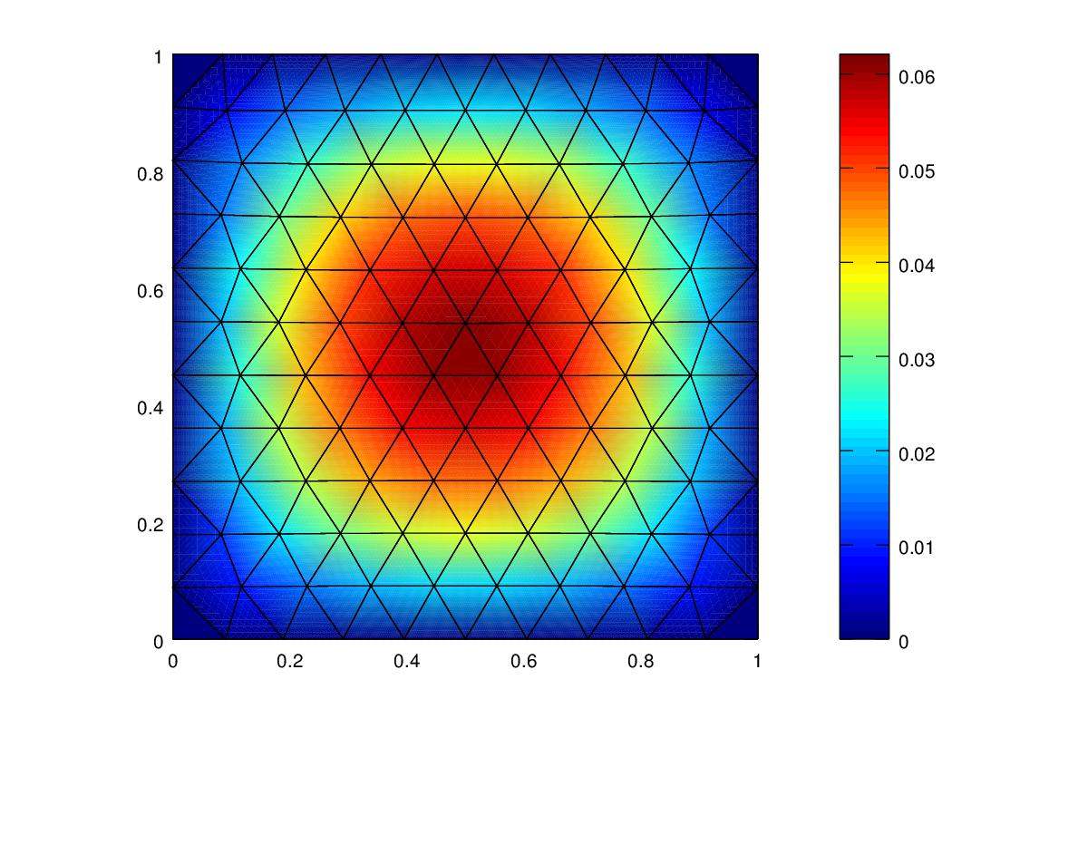
In this experiment we will solve Poisson’s equation over a square region using Finite Elements with linear, quadratic and cubic elements and compare the results. We will solve
$$ -\nabla \cdot (k(x,y) \nabla u(x,y)) = f(x,y)$$
over a 2D square shape going from lower left coordinates (0,0) to upper right coordinates (1,1) with dirichlet boundary conditions of zero. The known solution for u(x,y) with zero boundary conditions on the square is
$$ u(x,y) = xy(1-x)(1-y)$$
We will also set the value of k(x,y) in the partial differential equation to
$$ k(x,y) = 1 + xy^2$$
taking the derivative of u with respect to x and y
$$ \dfrac{\partial u}{\partial x} = y-y^2-2xy+2xy^2 \\[0.3em] \dfrac{\partial u}{\partial y} = x-2xy-x^2+2x^2y$$
Plugging these equations into equation Poisson’s equation above and you get the following for f(x,y)
$$ f(x,y) = y^4-y^3+4y^3x-4y^4x+2y-2y^2-2x^2y+6x^2y^2+2x^3y-6x^3y^2+2x-2x^2$$
Since $$ u(x,y) $ is the known solution I can plot it below and compare it with the Finite Element approximation to \(u(x,y) \).
The Finite Element Method is designed to minimize the Energy Norm
$$ \text{Energy Norm} = (\iint k*(\nabla U^* – \nabla u^*)^2\,{d}A)^{1/2}$$
which may not result in the lowest displacement norm L2.
$$ \text{L2 Norm} = (\iint (U^* – u^*)^2\,{d}A)^{1/2}$$
Where \( U^*\) is the best solution from Finite Elements and \(u^*\) is the exact solution.
The P1, P2 and P3 Finite Element Codes in Matlab for this experiment can be found here:
These codes used the Matlab code from the previous post as a starting point which I modified to incorporate the equations of this experiment and to implement quadratic and cubic Finite Element algorithms. I also added code to calculate the Energy Norm and L2 Norm. In the quadratic case I added code to generate 3 additional mesh points per triangular element and also used a three point gauss quadrature rule to evaluate the integral over the triangle.
For the Cubic finite element code I added 7 additional nodes per triangle element and made use of a 6 point gauss quadrature rule to evaluate the integral in calculating K and F. You can find out more about using guass quadrature to evaluate integrals over a triangle in section 6.3 of this document.
The results of experiment 1 are shown in the following table:
| Polynomial | Mesh Resolution | Energy Norm | Energy Norm % error | L2 Norm |
|---|---|---|---|---|
| Linear | 0.1 | 0.021847 | 13.54 | 0.0012522 |
| Quadratic | 0.1 | 0.00067438 | 0.418 | 3.77e-5 |
| Cubic | 0.1 | 0.0000184 | 0.011 | 3.4e-6 |
Refining the mesh resolution produces the following:
| Polynomial | Mesh Resolution | Energy Norm | Energy Norm % error | L2 Norm |
|---|---|---|---|---|
| Linear | 0.05 | 0.010054 | 6.23 | 4.4e-4 |
| Quadratic | 0.05 | 0.000155 | 0.09 | 6.75e-6 |
| Cubic | 0.05 | 0.00000196 | 0.0012 | 3.8e-7 |
As can be seen from the above table the Cubic elements produced the most accurate approximation to the exact solution both in terms of the Energy Norm and the L2 Norm. Refining the mesh produced more accurate results for all polynomials. Notice that the quadratic results from the original mesh are still more accurate than the linear results on the refined mesh. The accuracy of the coarser cubic mesh results were about the same level of accuracy as than the refined quadratic mesh results.
Experiment 2
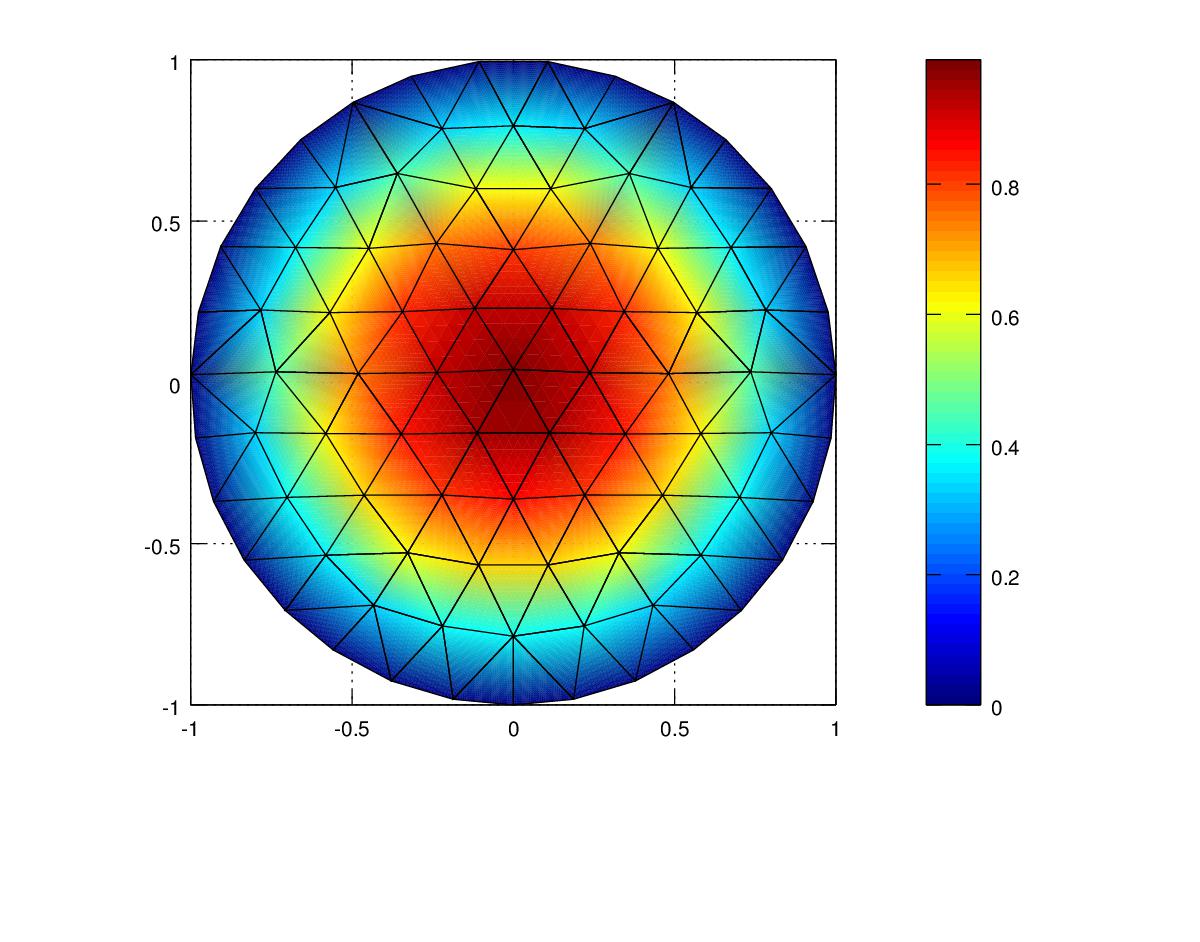
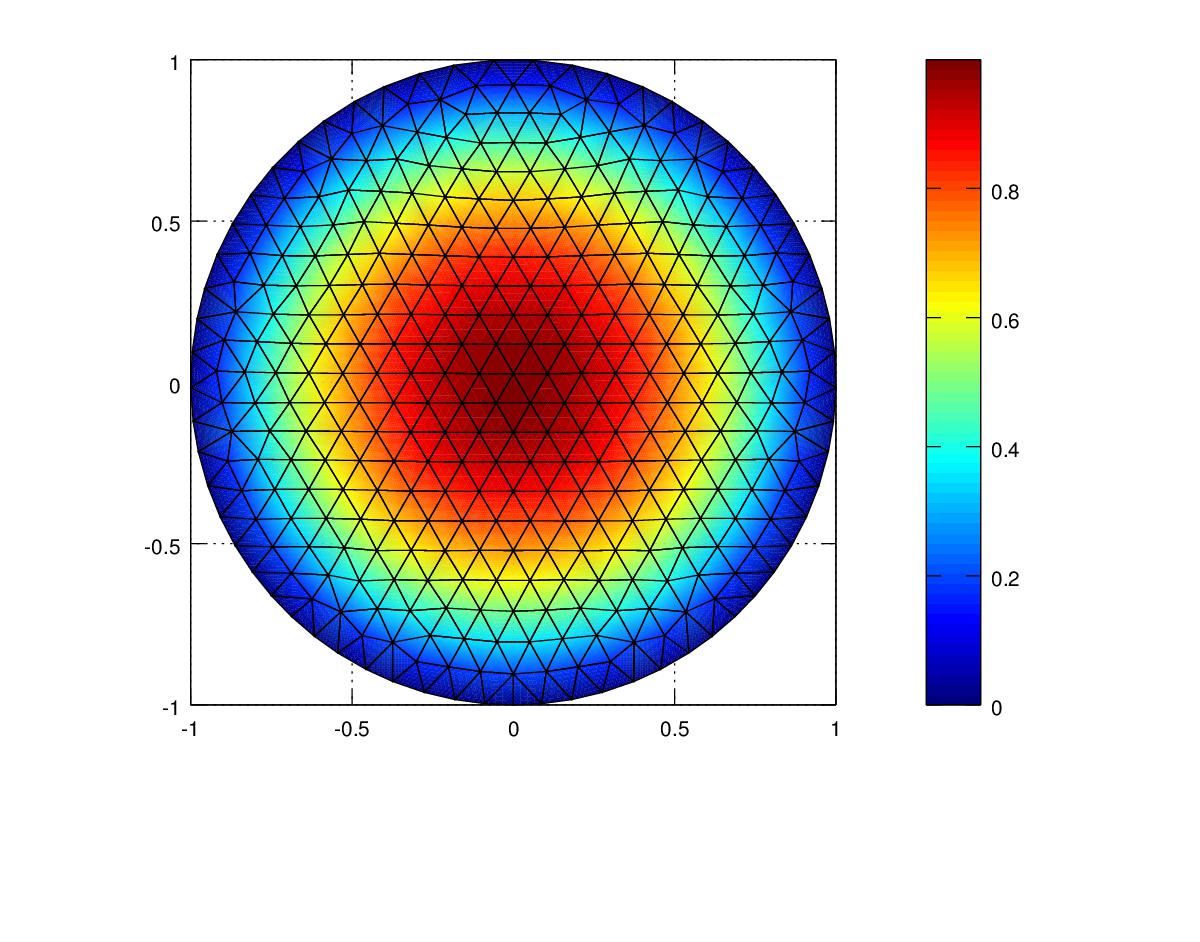
In this experiment we will solve Poisson’s equation over the unit circle and compare the results.
$$ -\nabla \cdot (k(x,y) \nabla u(x,y)) = f(x,y)$$
The exact solution for u(x,y) with zero boundary conditions on the unit circle is
$$ u(x,y) = 1 – x^2 – y^2$$
We will also set the value of k(x,y) in the partial differential equation to
$$ k(x,y) = 1$$
Taking the derivative of u with respect to x and y we get
$$ \dfrac{\partial u}{\partial x} = -2x \\[0.3em] \dfrac{\partial u}{\partial y} = -2y$$
Plugging these equations into Poisson’s equation above I get the following for f(x,y)
$$ f(x,y) = 4$$
The P1, P2 and P3 Finite Element Codes in matlab for this experiment can be found here:
The results of experiment 2 are shown in the following images and tables.
| Polynomial | Mesh Resolution | Energy Norm | Energy Norm % error | L2 Norm |
|---|---|---|---|---|
| Linear | 0.2 | 0.24225 | 9.73 | 0.015644 |
| Quadratic | 0.2 | 0.071976 | 2.89 | 0.055831 |
| Cubic | 0.2 | 0.051905 | 2.08 | 0.053181 |
Refining the mesh resolution produced the following:
| Polynomial | Mesh Resolution | Energy Norm | Energy Norm % error | L2 Norm |
|---|---|---|---|---|
| Linear | 0.1 | 0.10871 | 4.3 | 0.0073 |
| Quadratic | 0.1 | 0.025 | 1.0 | 0.0327 |
| Cubic | 0.1 | 0.018832 | 0.75 | 0.032 |
For this experiment the Cubic elements produced the lowest Energy Norm error value of 2% followed by the quadratic at 2.89% and Linear at 9.73% for the original mesh. For the refined mesh the Energy Norm was below 1 percent for Quadratic and Cubic polynomials The Linear element resulted in lowest L2 Norm followed by the Cubic L2 norm and then the Quadratic L2 norm. This result shows that the Finite Element algorithm is designed to minimize the Energy Norm and not the displacement norm or mean square error.
In this experiment, the accuracy did not improve as much as it did in Experiment 1 when using a higher order polynomial. This is due to the fact that we are using a triangular shaped mesh to approximate the curved boundary. When you have a polygonal domain such as a rectangle or square, this can be triangulated exactly with a triangular mesh leading to highly accurate solutions with higher order polynomials. In the case of a curved domain, we can only approximate its shape with a polygonal mesh and this introduces some error in the solution. The cubic polynomial solution on the curved boundary gave only a small improvement in accuracy compared to the quadratic polynomial solution. In Experiment 1 the improvement in accuracy was much greater when going from quadratic to cubic polynomial.
Experiment 3
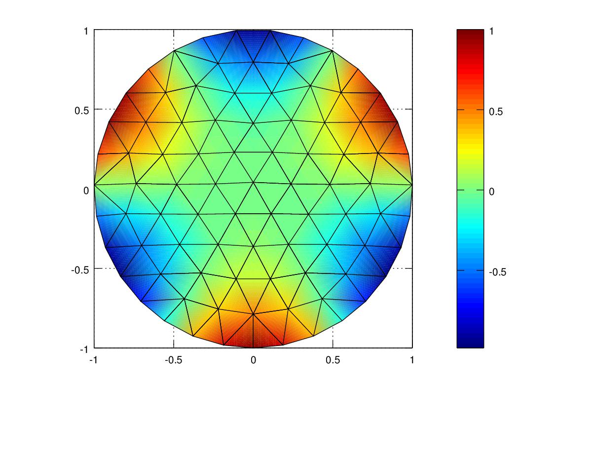
In this experiment we will solve Laplace’s equation over the unit circle with nonzero boundary conditions and compare the results.
$$ -\nabla \cdot (k(x,y) \nabla u(x,y)) = f(x,y)$$
The known solution is
$$ u(x,y) = 3yx^2-y^3$$
We will also set the value of k(x,y) in the partial differential equation to
$$ k(x,y) = 1$$
taking the derivative of u with respect to x and y
$$ \dfrac{\partial u}{\partial x} = 6yx \\[0.3em] \dfrac{\partial u}{\partial y} = 3x^2 – 3y^2$$
Plugging these equations into the differential equation I get the following for f(x,y)
$$f(x,y) = 0$$
which is what you expect for a Laplace equation. The boundary condition around the unit circle at radius 1.0 is set to \(sin(3\theta)\).
The P1, P2 and P3 Finite Element Codes in matlab for this experiment can be found here:
The results of experiment 3 are shown in the following images and tables.
| Polynomial | Mesh Resolution | Energy Norm | Energy Norm % error | L2 Norm |
|---|---|---|---|---|
| Linear | 0.2 | 0.72147 | 23.7 | 0.035458 |
| Quadratic | 0.2 | 0.088316 | 2.9 | 0.021873 |
| Cubic | 0.2 | 0.065215 | 2.1 | 0.01978 |
Refining the mesh produced the following:

| Polynomial | Mesh Resolution | Energy Norm | Energy Norm % error | L2 Norm |
|---|---|---|---|---|
| Linear | 0.1 | 0.32671 | 10.6 | 0.00875 |
| Quadratic | 0.1 | 0.028789 | 0.94 | 0.015991 |
| Cubic | 0.1 | 0.021882 | 0.714 | 0.015 |
In this experiment the Cubic elements produced the most accurate results both in terms of Energy Norm and L2 Norm, followed by quadratic elements and then linear elements. With the refined mesh, the Cubic polynomial produced the most accurate result in terms of Energy Norm but the Linear polynomial had the lowest L2 norm. Due to the error introduced by approximating the curved boundary by a polygonal mesh, the higher order polynomials did not improve the accuracy of the solution by any significant amount. Reference 5 in the references provided below explains that the accuracy of Finite Elements on curved boundaries can be improved by using “Isoparametric quadratic triangles” or by using a nonuniform mesh with smaller elements near the curved boundary.
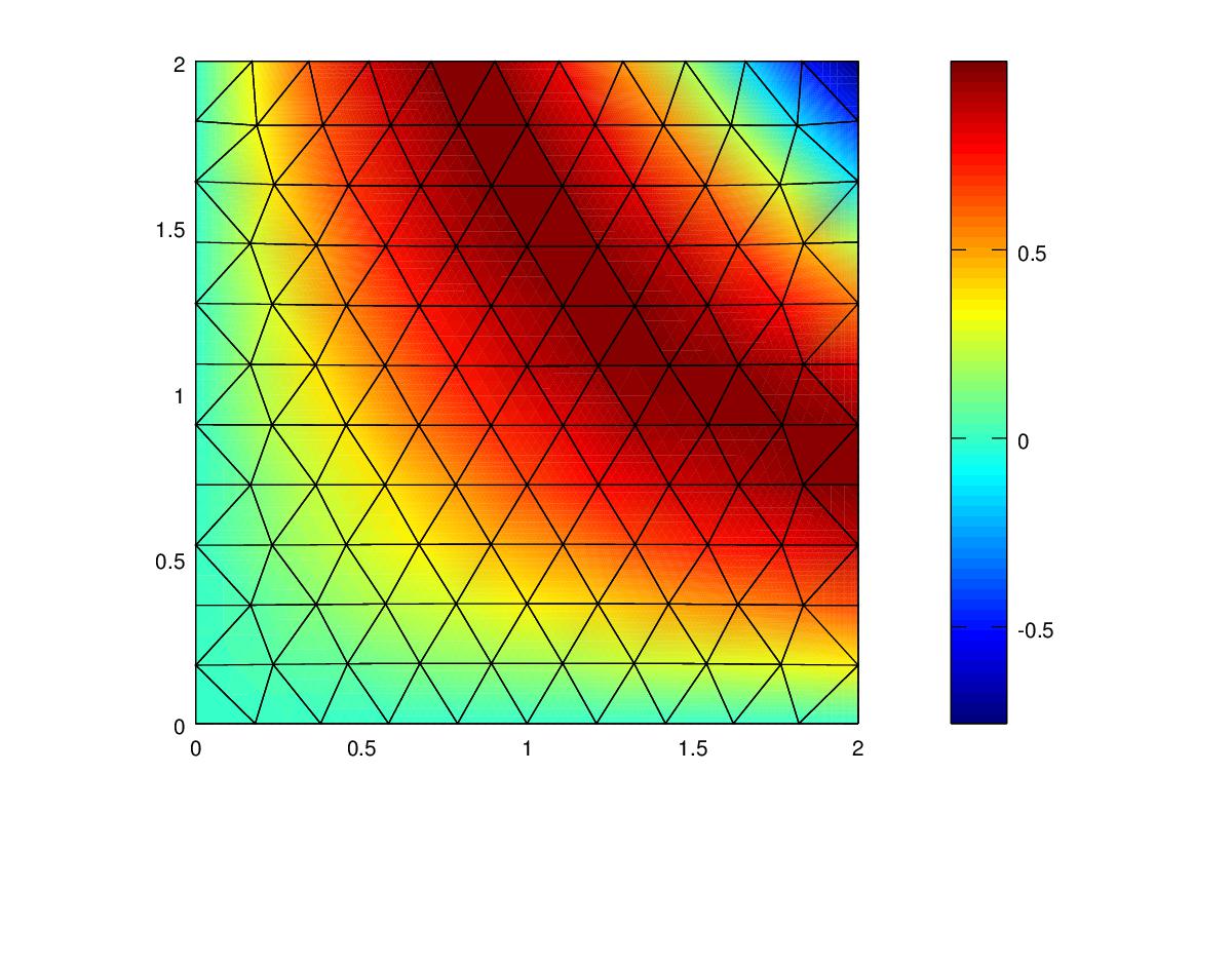
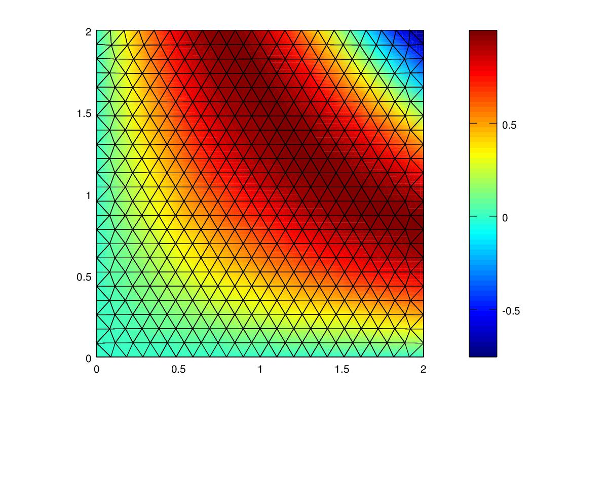
Experiment 4
In this experiment we will solve Laplace’s equation over a square with nonzero boundary conditions along 2 sides and compare the results.
$$ -\nabla \cdot (k(x,y) \nabla u(x,y)) = f(x,y)$$
The known solution is
$$ u(x,y) = \sin(xy)$$
We will also set the value of k(x,y) in the partial differential equation to
$$ k(x,y) = 1$$
taking the derivative of u with respect to x and y
$$ \dfrac{\partial u}{\partial x} = y\cos(xy) \\[0.3em]\dfrac{\partial u}{\partial y} = x\cos(xy)$$
Plugging these equations into the differential equation I get the following for f(x,y)
$$ f(x,y) = y^2\sin(xy) + x^2\sin(xy)$$
The boundary condition around the square shape from (0,0) to (2,2) are as follows:
$$ u(0,y) = 0 \\[0.3em] u(x,0) = 0\\[0.3em] u(2,y) = \sin(2y)\\[0.3em] u(x,2) = \sin(2x)\\[0.3em]$$
The P1, P2 and P3 Finite Element Codes in matlab for this experiment can be found here:
The results of experiment 4 are shown in the following images and tables.
| Polynomial | Mesh Resolution | Energy Norm | Energy Norm % error | L2 Norm |
|---|---|---|---|---|
| Linear | 0.2 | 0.26774 | 11.52 | 0.011972 |
| Quadratic | 0.2 | 0.0091104 | 0.392 | 4.82e-4 |
| Cubic | 0.2 | 0.00044193 | 0.019 | 6.88e-5 |
Refining the mesh produced the following:
| Polynomial | Mesh Resolution | Energy Norm | Energy Norm % error | L2 Norm |
|---|---|---|---|---|
| Linear | 0.1 | 0.12835 | 5.523 | 0.0046242 |
| Quadratic | 0.1 | 0.0021472 | 0.092396 | 9.449e-5 |
| Cubic | 0.1 | 0.0000481 | 0.00207 | 8.293e-6 |
This Experiment produced similar results to Experiment 1. For both meshes, the Cubic elements produced the most accurate results both in terms of Energy Norm and L2 Norm, followed by quadratic elements and then linear elements. Note that the cubic polynomial from the original mesh produced more accurate results than both the linear and quadratic polynomials did in the refined mesh.
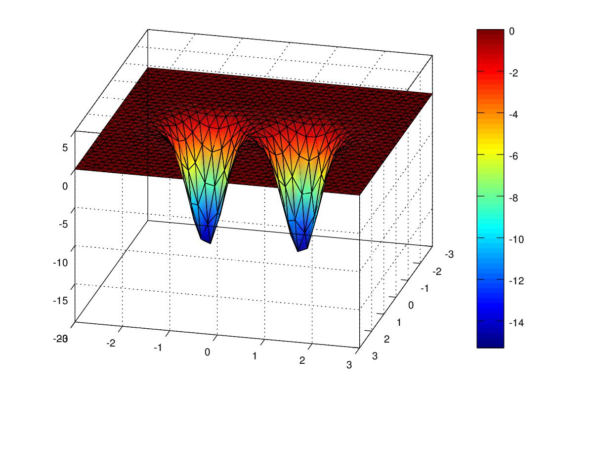
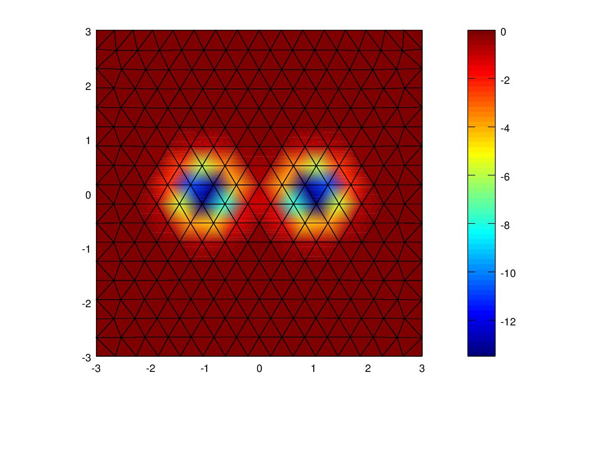
Experiment 5
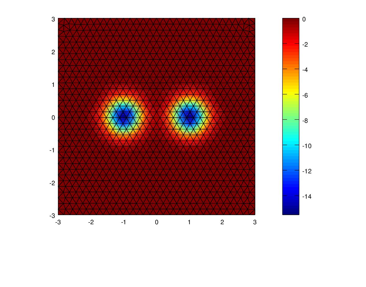
In this experiment we will solve Poisson’s equation over a square with zero boundary conditions and a known solution containing an exponential function.
$$ -\nabla \cdot (k(x,y) \nabla u(x,y)) = f(x,y)$$
The known solution is
$$ u(x,y) = -16*\exp(-4*((x-1)^2 + y^2)) – 16*\exp(-4*((x+1)^2 + y^2));$$
We will also set the value of k(x,y) in the partial differential equation to
$$ k(x,y) = 1$$
taking the derivative of u with respect to x and y
$$ \dfrac{\partial u}{\partial x} = 64*(2*x-2)*\exp(-4*((x-1)^2 + y^2)) + 64*(2*x+2)*\exp(-4*((x+1)^2 + y^2)) \\[0.3em] \dfrac{\partial u}{\partial y} = 64*2*y*\exp(-4*((x-1)^2 + y^2)) + 64*2*y*\exp(-4*((x+1)^2 + y^2))$$
Plugging these equations into the differential equation I get the following for f(x,y)
$$ f(x,y) = -128*\exp(-4*((x-1)^2 + y^2)) – 128*(x-1)*(-8*(x-1))*\exp(-4*((x-1)^2 + y^2)) – 128*\exp(-4*((x-1)^2 + y^2)) – 128*y*(-4*2*y)*\exp(-4*((x-1)^2 + y^2)) -128*\exp(-4*((x+1)^2 + y^2)) – 128*(x+1)*(-8*(x+1))*\exp(-4*((x+1)^2 + y^2)) – 128*\exp(-4*((x+1)^2 + y^2)) – 128*y*(-4*2*y)*\exp(-4*((x+1)^2 + y^2))$$
This solution is plotted in 3D below.
The P1, P2 and P3 Finite Element Codes in matlab for this experiment can be found here:
The results of experiment 5 are shown in the following images and tables.
| Polynomial | Mesh Resolution | Energy Norm | Energy Norm % error | L2 Norm |
|---|---|---|---|---|
| Linear | 0.4 | 16.303 | 40.693 | 1.9347 |
| Quadratic | 0.4 | 2.2814 | 5.69 | 0.57639 |
| Cubic | 0.4 | 0.35742 | 0.89 | 0.056748 |
Refining the mesh produced the following:
| Polynomial | Mesh Resolution | Energy Norm | Energy Norm % error | L2 Norm |
|---|---|---|---|---|
| Linear | 0.2 | 8.154 | 20.355 | 0.78274 |
| Quadratic | 0.2 | 0.50496 | 1.26 | 0.0744 |
| Cubic | 0.2 | 0.042839 | 0.106 | 0.0122 |
| Polynomial | Mesh Resolution | Energy Norm | Energy Norm % error | L2 Norm |
|---|---|---|---|---|
| Linear | 0.1 | 4.0267 | 10.052 | 0.36784 |
| Quadratic | 0.1 | 0.11769 | 0.2938 | 0.00886 |
| Cubic | 0.1 | 0.005144 | 0.012842 | 0.00167 |
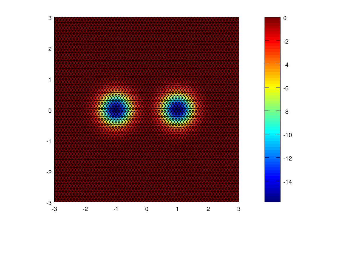
For this experiment, on the course mesh the Energy norm error of the linear polynomial was 40% but that of the cubic polynomial was below 1%. I added an extra table refining the mesh further. For the linear case, reducing the mesh spacing from 0.4 to 0.2 to 0.1 resulted in halving the Energy Norm for each step. For the quadratic polynomial the Energy Norm was over 4 times less for each step. For the cubic polynomial the Energy Norm was over 8 times less for each step.
Summary
- Piecewise Polynomials are used in the Finite Element method to approximate solutions to partial differential equations.
- The Finite Element method minimizes the Energy Norm when it solves Poisson’s or Laplace’s equation.
- Using higher order polynomials results in more accurate solutions in the Energy Norm sense.
- A shape with a polygonal boundary that is approximated with a polygonal mesh results in highly accurate solutions when using higher order polynomials.
- A shape with a curved boundary that is approximated with a polygonal mesh introduces errors along the boundary and the improvement in accuracy is much less pronounced when using higher order polynomials.
- Isoparametric quadratic triangles as explained in Reference 5 can be used in Finite Elements to improve the accuracy of for domains with curved boundaries.
References
- Section 3.6 The Finite Element Method in the book “Computational Science and Engineering” by Gilbert Strang
- Section 5.4 The Finite Element Method in the book “Introduction to Applied Mathematics” by Gilbert Strang
- DistMesh – A Simple Mesh Generator in MATLAB
- Finite Elements in 2D video lecture.
- Understanding and Implementing the Finite Element Method by Mark S. Gockenback
Below are two emails from John describing some further work he has done with these codes. I decided to post these here since I think most of you will find them relevant.
Hi Lubos
I tried replacing the built in MATLAB solver with the Conjugate Gradient algorithm for the P1, P2, P3 files used in Experiment 1 and it gave me the exact same solutions as the built in solver. Here is the Conjugate Gradient version of femcode_P1
http://dl.dropbox.com/u/5095342/fempoisson/Experiment1/femcode_cg_P1.m.htm
All I did was comment out the line for the built in MATLAB solver
%U=Kb\Fb; % The FEM approximation is U_1 phi_1 + ... + U_N phi_Nand replaced it with the following CG algorithm.
This worked fine for Experiment1 samples but for some of the other experiments it did not work so well. It seems like the built in MATLAB solver has a lot of techniques at its disposal when solving the linear system KU=F because it found more accurate solutions in some Experiments when the CG algorithm either failed or returned a less accurate solution.
Hi again
I looked into the conjugate gradient a little further. I get it to work in place of the built in MATLAB solver for all the Experiments now provided the matrix K from KU=F is well conditioned. I also needed to change my code a little for experiments where the dirichlet boundary condition is non zero. For instance, in Experiment3 I changed the code in femcode_P1 when setting up the boundary conditions to the following.
http://dl.dropbox.com/u/5095342/fempoisson/Experiment3/femcode_P1a.m.htm
and the version with the conjugate gradient solver for this is here.
http://dl.dropbox.com/u/5095342/fempoisson/Experiment3/femcode_cg_P1a.m.htm
So now provided the matrix K is well conditioned, the conjugate gradient solver works each time. I guess that the built in matlab solver will handle ill conditioned K matrices correctly whereas the conjugate gradient algorithm I provided will fail if the condition number of the K matrix is too high.
John
Hi,
i am cyrille student at university of Padova i am interesting in the solution of Poisson equation with Nonzero Dirichlet BC using the Conjuguate Gradient Method and the comments found in this blog were precious to move on my task, but i need help to finish.
John posted his recent work on the CG method and he has sent us to the link that i attached above in website position, the problem is that the informations is not availables anymore. Could anyone give me and example of codes allowing to solve Poisson Equation with non zero Dirichet Boundary Condition using Comjuguate Gradient Method? or does anyone still have the code published by John in that blog?
Thanks you for yours anwers
Regards
Attached are links to the requested files via dropbox service.
https://www.dropbox.com/s/uqvkv0s2ole2e6u/femcode_cg_P1a.m.htm?dl=0
https://www.dropbox.com/s/b8a5t1g89ndg8pp/femcode_P1a.m.htm?dl=0
You might need a dropbox account to view the files now. Dropbox changed how to access public files and that is why the original links no longer worked.
Further with regard to the issue of condition number of the matrix K and the conjugate gradient method. If the condition number gets too high then you need to use a Preconditioned Conjugate Gradient algorithm. What I found was that when the mesh used for the domain in the Finite Element Method became too large from being too refined then the condition number of the assembled stiffness matrix K would become large and the simple conjugate gradient would not work as a solver. However, the preconditioned conjugate gradient algorithm, which reduces the condition number of K, always works as a solver for Finite Elements. Matlab has a built in function called pcg for preconditioned conjugate gradient which can be used instead of the standard solver that matlab contains. More information can be found at the following links.
http://www.mathworks.com/help/techdoc/ref/pcg.html
http://www.math.iit.edu/~fass/477577_Chapter_16.pdf
its nice thankyou
I am doing Phd from NIT hamirpur India. I am working on matlab in FEM. I want to develop Stiffness matrix(1D) using rayleigh ritz method(Min. energy approach). As i am relatively new in matlab coding, can anyone suggest me how to proceed?
There are some sample matlab codes on this web page from the book Computational Science and Engineering.
http://math.mit.edu/~gs/cse/
Just scroll down to see some sample matlab codes for content from the book.
I guess you just need to learn matlab.
Here are a couple if lectures on FEM in 1D from the author of the book.
https://ocw.mit.edu/courses/mathematics/18-085-computational-science-and-engineering-i-fall-2008/video-lectures/lecture-17-finite-elements-in-1d-part-1/
https://ocw.mit.edu/courses/mathematics/18-085-computational-science-and-engineering-i-fall-2008/video-lectures/lecture-18-finite-elements-in-1d-part-2/
John
Hi professor ,I have a question, if i want to caculate the potential of a rectangle region, this area have two electrodes, the upper electrode(100V) and the lower electrode(20V). The length is 3cm, the width is 3cm, DR=1cm, DZ=1cm. I’m a little confused which kind of boudary is correct?
1). 4*4 nodes
0 0 0 0 —-> upper electrode (100V)
0 0 0 0
0 0 0 0
0 0 0 0 —-> lower electrode (20V)
2). 5*5 nodes
0 0 0 0 0->upper electrode (100V)
0 0 0 0 0
0 0 0 0 0
0 0 0 0 0
0 0 0 0 0
0 0 0 0 0 ->lower electrode (20V)
i made a mistake in case 2 5*5 nodes, it should be 5*5, i
drawed into 6*5, sorry.
Hello everyone,
I am currently on a heat transfer equation PDE using 2D hexagonal meshing, does anyone have any idea on how to figure out the shape functions and how to compute and plot them
Thank u
Best regards from Morocco
You can do this fairly easily using the Finite Volume Method.
Hello,
I want yo Solver The Poisson Equation in 2D on the Unit Circle with finite Elements. My problem is the computation of the order of convergence. From the a priori Theorem the L2 error should be 2 but in the code above the exact solution is interpolated at the nodes and every time when I change the h it changes the reference element. My problem is that the Interpolation of the exact solution is not so good to show the theorem. What else can I do instead to approximate the order of convergence?