Starfish Tutorial Part 2: Particles and Animation

Introductions
This is the second part of the Starfish plasma simulation code tutorial. We will continue with the example started in Part 1. Our goal is to model the flow of plasma over an infinitely long cylinder (since Starfish is a two-dimensional code). In the last example, we set up the computational domain, specified the cylinder geometry, and used the Poisson solver to compute the initial potential. In this example we add particles. We also discuss how to generate animations.
Adding Particles
In order to add particles, we need to specify sources. Starfish supports two types: volumetric and surface based. We will use the latter. Surface sources create particles along geometry splines according to a prescribed velocity distribution function (VDF) and the surface normal vector. We want the entire left domain boundary to act as a source injecting particles with uniform velocity. This setup then approximates the movement of the cylinder through undisturbed plasma, with the frame of reference moving with the cylinder. First, we need to add a new boundary to the boundaries.xml file:
<boundaries>

<boundary name="cylinder" type="solid" value="-1">
<material>SS</material>
<path>M 0.05, 0 L 0.0475528, -0.0154508 0.0404508, -0.0293893 0.0293893, -0.0404508 0.0154508, -0.0475528 -9.18E-18, -0.05 -0.0154508, -0.0475528 -0.0293893, -0.0404508 -0.0404508, -0.0293893 -0.0475528, -0.0154508 -0.05, 6.12E-18 -0.0475528, 0.0154508 -0.0404508, 0.0293893 -0.0293893, 0.0404508 -0.0154508, 0.0475528 3.06E-18, 0.05 0.0154508, 0.0475528 0.0293893, 0.0404508 0.0404508, 0.0293893 0.0475528, 0.0154508 0.05, 0</path>
</boundary>

<boundary name="inlet" type="virtual">
<path>M -0.15,0.20 L -0.15, 0</path>
</boundary>

</boundaries>
We named this spline “inlet” and gave it a virtual type. This classification means that the boundary will not be used to set potential and will not be seen by the particles. However, it is available for use by sources and by probes. This spline is simply a linear segment between the top left and bottom left corner of the computation mesh. Starfish uses the right hand rule to set the normal vector, and hence the line goes from top to bottom. Particles are generated in the normal direction so the normal needs to be pointing in the +x direction. The line is 0.2m long.
To add the source, we add the following command to starfish.xml (this command could also be placed in an external file and loaded with the load command):
<!-- set sources -->
<sources>
<boundary_source name="space">
<type>uniform</type>
<material>O+</material>
<boundary>inlet</boundary>
<mdot>3.72e-13</mdot>
<v_drift>7000</v_drift>
</boundary_source>
</sources>
Here you can see how the boundary comes into play. The source is given type uniform, which means that it produces particles with velocity equal to v_drift. The particles will be moving in the direction of the surface normal of the associated boundary. If the boundary consisted of a number of individual splines, the particles would be injected according to the local normal.
This source will generate O+ particles at mass flow rate of 3.72e-13 kg/s. You may be wondering how this number was determined. We want our plasma density in the free space to be \(10^{10}\, \text{m}^{-3}\), to correspond with the potential solver electron model settings. The mass flow rate is given by the following expression:
$$\dot{m}=m n u A$$
where the terms on the RHS correspond to the atomic mass (16 amu, per materials.xml file), number density (1e10 m-3), velocity (7,000 m/s), and source area (0.2 m2). In the Cartesian (XY) mode, the area is equal to the spline length, since unit depth is assumed. This expression gives us the value that is used in the simulation.
Also, since we now have particles, we need to run for enough time steps to reach the steady state. In this case, 400 time steps will do the trick. We modify the time command as follows:
<!-- set time parameters -->
<time>
<num_it>400</num_it>
<dt>1e-7</dt>
</time>
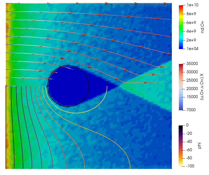
And that’s it. You will find the complete set of input files in the step2 subfolder. After we run the simulation, we obtain the results shown below. We can see that a wake forms behind the cylinder. We can also clearly see the “reflection” of ions at the centerline, the line of symmetry. In reality, this reflection corresponds to the influx of particles from the opposite half of the simulation. This is best seen in the plot of the vertical velocity.
Animations
The above results show the final solution at the end of the simulation. These results correspond to the instantaneous steady state results. But what if we wanted to learn more about how the solution progressed? Or what if we had a time-dependent injection source? This is where animations come in. Animations direct the simulation to save results at a prescribed frequency during the course of the computation. Animations are specified by wrapping the standard output command in an animation command:
<!-- save animation -->
<animation start_it="1" frequency="10">
<output type="2D" file_name="results/field_ani.vts" format="vtk">
<scalars>phi,rho, nd.O+, t.o+</scalars>
<vectors>[u.O+,v.O+]</vectors>
</output>
</animation>
The animation command is basically a wrapper for output, calling the specified output at a prescribed frequency. Here we start the animation with time step 1, and generate a file every 10 time steps.
More Fun with Starfish: Constant Electric Field
Finally, a bit more fun with Starfish. The Poisson solver is just one of many solvers available in the simulation. One of the other “solvers” is a constant electric field model. Instead of solving for plasma potential self consistently, this model simply specifies uniform electric field components everywhere in the domain. We can use this model to create an electric field directing ions toward the centerline.
<solver type="constant-ef">
<comps>0,-500</comps>
</solver>
Since the ions already have an initial horizontal velocity, this results in an interesting waterfall-like response, especially around the cylinder. We can also clearly see that density decreases as velocity increases, as expected.
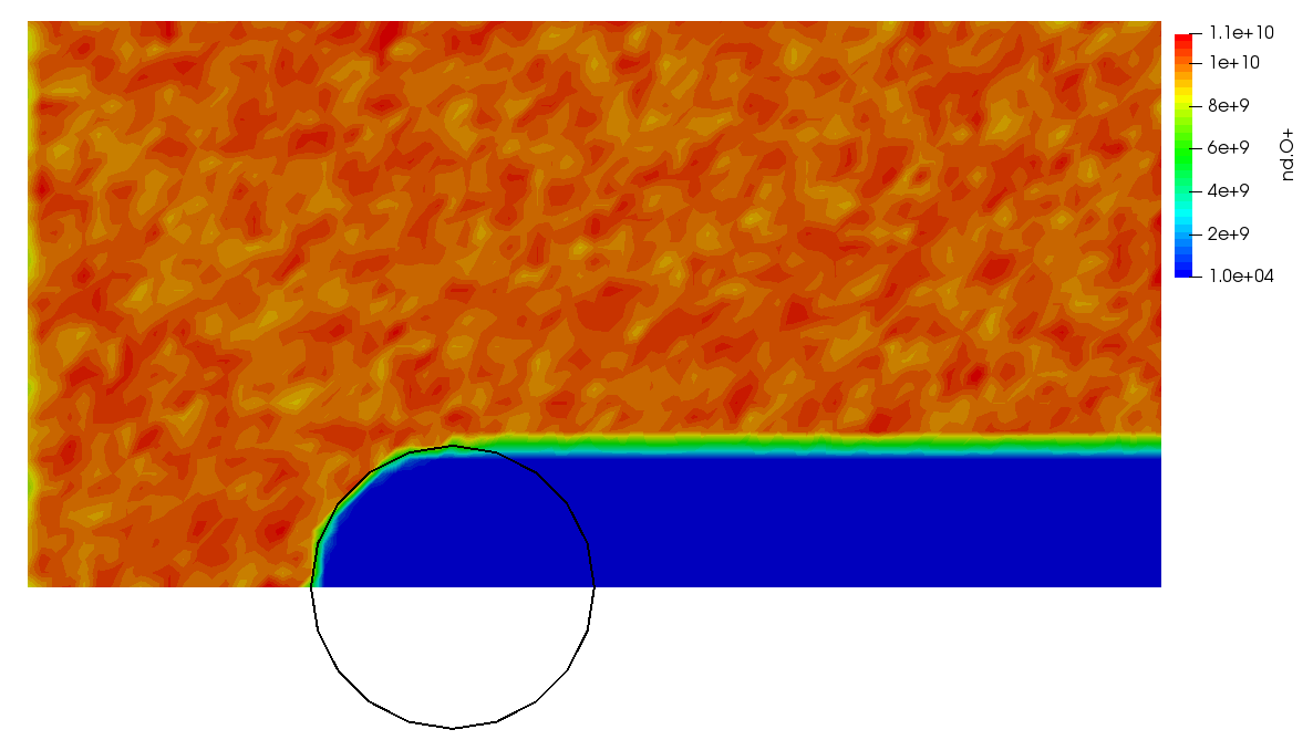
We can also use completely turn of the Poisson solver by commenting it out, or by using 0,0 for the constant electric field solver. This is especially useful for testing the particle injection source. We can see this in Figure 4. Since the field solver is turned off, the ions effectively act like neutral particles. We can see that the injected density is indeed the desired 1010 m-3.
Continue to Starfish Tutorial Part 3.