Starfish Tutorial Part 1: Domain, Boundaries, and a Potential Solver

Posted on October 29th, 2012
Previous Article :: Next Article

Starfish Tutorial

Starfish is a PIC-C developed 2D XY or RZ code for simulating plasmas and rarefied gases. Starfish will eventually contain a GUI that will simplify setting up simulation cases. However, for now, the code consists solely of an input file driven solver. In this five-step tutorial we will guide you through the steps used to setup a representative simulation. The simulation investigates the flow of plasma over a charged cylinder, and considers erosion of the cylinder due to ion bombardment. In this first lesson, we will go through the steps needed to specify the computational domain, add the geometry (the cylinder), solve the potential, and output results.

Running Starfish

Starfish is a Java application and in order to run it, you will need to have the Java run time environment installed. You will also need the input files, which you will find in the dat/tutorial directory included with the Starfish distribution.

It is possible that your machine already associates .jar files with Java. If so, you may be able to start the code by copying the .jar file into the simulation folder and double clicking on it. Alternatively, you can launch the solver from the command line. Use your operating system specific instructions to navigate to the folder containing your input files. For instance, on Microsoft Windows 7, you could start the command prompt by pressing “Windows Key + R” and typing cmd into the dialog box. Then use the cd command to reach the target directory. There type in java -jar starfish.jar to launch the code. If everything went well, you will see:

C:\codes\starfish\dat\tutorial\step1>java -jar starfish.jar
================================================================
> Starfish v0.20.1 (Development)
> 2D Plasma / Rarefied Gas Simulation Code
> (c) 2012-2019, Particle In Cell Consulting LLC
> info@particleincell.com, www.particleincell.com
 
!! This is a development version. The software is provided as-is, 
!! with no implied or expressed warranties. Report bugs to 
!! bugs@particleincell.com
=================================================================
Processing <note>
**Starfish Tutorial: Part 1**
Processing <domain>
Processing <materials>
Processing <boundaries>
Processing <solver>
Processing <time>
Processing <starfish>
Starting main loop
WARNING: The simulation failed to reach steady state!
Processing <output>
Processing <output>
Processing <output>
Done!

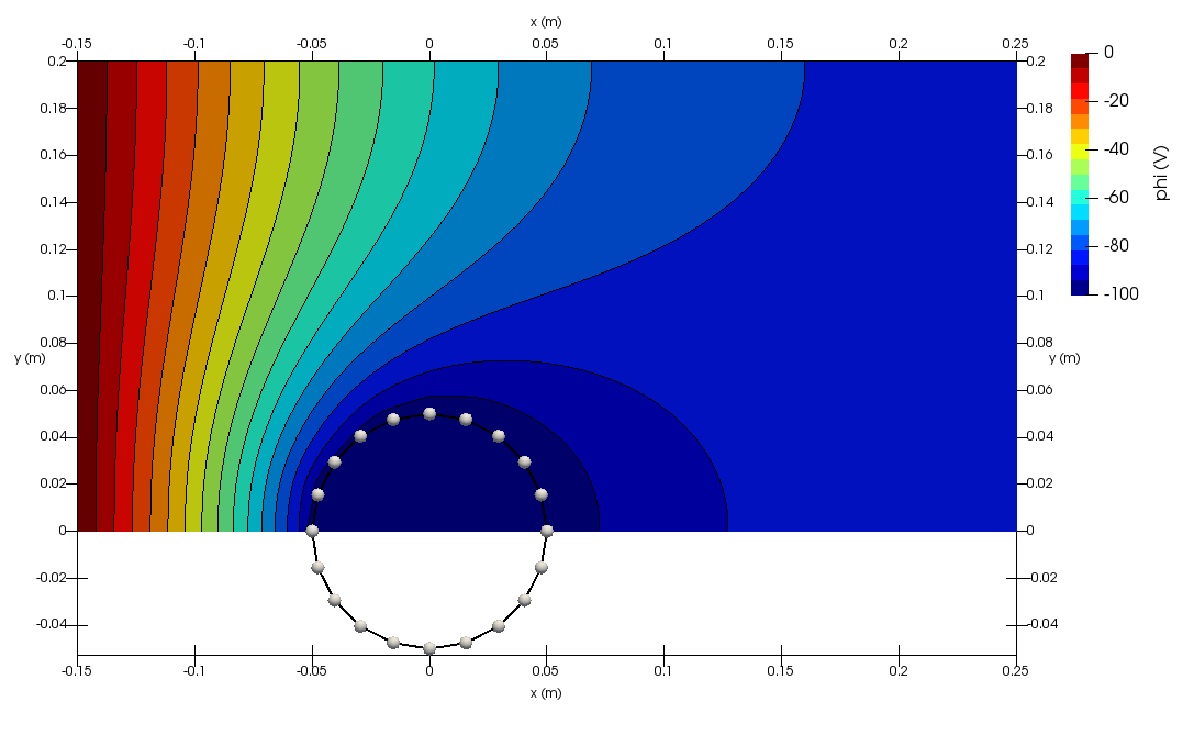
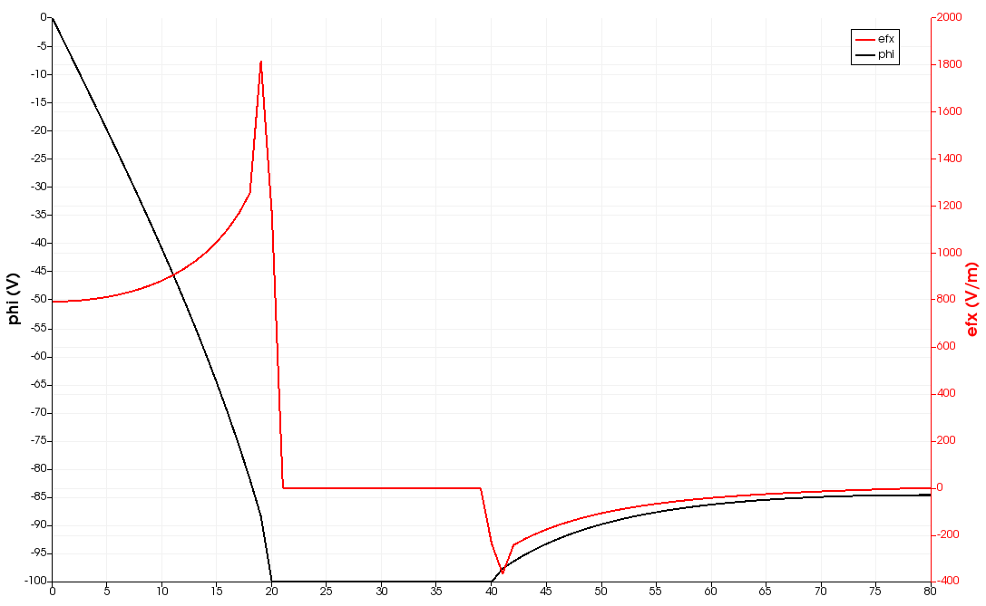
You will also see few new files appear in a results folder: boundaries.vtp, field.pvd, field_mesh1.vts, and profile.dat. These files contain various simulation outputs in a VTK format compatible with Paraview or Visit. Plots made from these files can be seen below in Figure 1. In addition, you will also find a log file starfish.log which contains some additional details.

2D potential plot — Figure 1. Some example simulation results. The first plot shows the 2D potential profile from `field.pvd` with the cylinder outline from `boundaries.vtp`. The second image shows the potential and efx along the y=0 line. The discontinuity is due to Starfish utilizing first-order differencing on geometry boundaries.

Figure 1. Some example simulation results. The first plot shows the 2D potential profile from `field.pvd` with the cylinder outline from `boundaries.vtp`. The second image shows the potential and efx along the y=0 line. The discontinuity is due to Starfish utilizing first-order differencing on geometry boundaries.

Starfish Input File (starfish.xml)

When Starfish is launched, it looks for a file named starfish.xml in the current directory. This file contains the commands that drive the simulation. The file used to produce the output in Figure 1 is shown below:

```
<simulation>    
```
```
<note>Starfish Tutorial: Part 1</note>
```
```
 
```
```

```
```
<load>domain.xml</load>
```
```
<load>materials.xml</load>
```
```
<load>boundaries.xml</load>
```
```
 
```
```

```
```
<solver type="poisson">
```
```
<method>gs</method>
```
```
<n0>1e10</n0>
```
```
<Te0>1.5</Te0>
```
```
<phi0>0</phi0>
```
```
<max_it>5e4</max_it>
```
```
</solver>
```
```
 
```
```

```
```
<time>
```
```
<num_it>0</num_it>
```
```
<dt>5e-7</dt>
```
```
</time>	
```
```
 
```
```

```
```
<starfish />
```
```
 
```

<!-- save mesh-based results in VTK format-->

<output type="2D" file_name="results/field.vts" format="vtk">

```
<scalars>phi, rho, nd.O+</scalars>
```
```
<vectors>[efi, efj]</vectors>
```
```
</output>
```
```
 
```

<!-- save data along a single mesh grid line -->

<output type="1D" file_name="results/profile.vts" format="vtk">

```
<mesh>mesh1</mesh>
```
```
<index>J=0</index>
```
```
<scalars>phi, rho, nd.o+</scalars>
```
```
<vectors>[efi, efj]</vectors>
```
```
</output>
```
```
 
```
```

```

<output type="boundaries" file_name="results/boundaries.vtp" format="vtk" />

```
 
```
```
</simulation>
```

As you can see, this is an XML document containing number of child elements nested within the parent <simulation> root element. Each XML element consists of an opening and a closing tag:

<starfish>
...
</starfish>

These can however be collapsed to a single line, which is especially handy for simpler commands:

<starfish />

XML documents can also contain comments:

<!-- this is a comment -->

Each element can contain children and/or attributes. Starfish does not distinguish between child nodes and attributes and it’s totally up to you how to provide the inputs. For instance, the commands below are identical:

<!-- command with child nodes -->
<time>
<num_it>0</num_it>
<dt>5e-7</dt>
</time>	
 
<!-- the same command with a mix of child nodes and attributes -->
<time num_it="0" />
<dt>5e-7</dt>
</time>	
 
<!-- the same command specified using only attributes -->
<time num_it="0" dt="5e-7" />

Line-by-Line Command Listing

Line 2: <note>

The input file starts with the note command, which simply outputs the specified message to the screen and the log file. This is a convenient way to remind you what simulation case the code is running.

Lines 5-7: <load>

The file next contains three load commands. These commands load the specified file and place it into the XML tree at the current position. They are used to split a single input file into more manageable smaller chunks. This command is particularly handy for data reuse, since you can load a file of commonly used materials and material interactions. We will go through the content of these in more detail below.

Lines 10-16: <solver>

Lines 10 through 16 contain the solver command. This command is used to specify the details of the solver that will be used in the simulation. Here we use the non-linear Poisson solver. The parameters specify the solution method (Gauss-Seidel), the reference values for the Boltzmann electron model, as well as the maximum number of iterations for the linear solver. Other parameters can also be set, such as the tolerance, and the settings for the non-linear NR solver, but here we just use the defaults. You can see the value of these by looking in the log file.

Lines 19-22: <time>

We next set time control parameters. We tell the code to run for a total of zero iterations. We also specify the time step size, which in this case is ignored. Running for zero iterations instructs the code to solve the initial field, but it will not attempt to inject particles (assuming sources were defined).

Line 24: <starfish>

On line 25 we finally start the simulation with the starfish command. All commands before this one were simply specifying the inputs, now these are used to compute the solution. The input file parser will wait for the solver to finish before moving to the next command.

Lines 28-42: <output>

By itself, the starfish command does not produce any useful output. The computed results are stored internally in memory data structures and must be saved to the output file. This is done with the output command. Three types of output are supported: 2D, 1D, and Boundaries. The first saves data on the 2D computational mesh. The 1D type is similar but it saves only a subset of the mesh along a fixed I or J grid line. The Boundaries output saves the simulation geometry. This plot is useful for outputting surface-type parameters such as erosion rate or surface flux. Here we use it to simply save the loaded object geometry. Here the data is stored in the VTK format with the electric field components grouped into a vector field.

Domain File (domain.xml)

We now return to line 5, and consider the domain specification. The domain file, domain.xml, contains the following:

<domain type="xy">
 
<mesh type="uniform" name="mesh1">
<origin>-0.15,0</origin>
<spacing>5e-3, 5e-3</spacing>
<nodes>81, 41</nodes>
<mesh-bc wall="left" type="dirichlet" value="0" />
<mesh-bc wall="bottom" type="symmetry"/>
</mesh>
</domain>

One of the unique features of Starfish is its ability to load an arbitrary number of computational meshes. These meshes can be either rectilinear or body fitted elliptic meshes. In this example, we specify just a single rectilinear mesh. However, we first tell the code that our geometry is in the Cartesian (XY) coordinate system. Starfish also supports axisymmetric (RZ) domains. The uniform Cartesian mesh is specified by providing the location of the origin, node spacing, and the number of nodes in the two coordinate directions. We also apply a mesh boundary condition by setting the left wall to a fixed 0V potential. This is needed in order to create a potential gradient between the ambient free space and the sphere.

Materials definition (materials.xml)

Starfish does not contain any build database of materials or material interactions. This information must be provided by the user. Since we don’t have any particles in this first step, we don’t yet concern ourselves with the interactions, however, we need to define the materials that will be present in the simulation. The materials file contains the following:

<!-- materials file -->
<materials>
 
<material name="O+" type="kinetic">
	<molwt>16</molwt>
	<charge>1</charge>
	<spwt>1e3</spwt>
	<init>nd_back=1e4</init>
</material>
 
<material name="SS" type="solid">
	<molwt>52.3</molwt> 
	<density>8000</density>
</material>
 
</materials>

As you can see, we defined two materials: atomic oxygen ions and stainless steel. The atomic oxygen ions are kinetic. This material will be modeled with simulation particles within the particle in cell method. Starfish also supports fluid materials, which use Navier Stokes or MHD equations to propagate densities, as well as solid materials, which don’t change throughout the simulation. The parameters needed to specify a material will depend greatly on the type of the material. For the kinetic oxygen ions, we specify the particle specific weight, or the number of real particles each simulation macroparticle represents. This number will influence the number of simulation particles in the simulation. We also specify the background density. A non-zero background density is required whenever the Boltzmann electron model is used due to the presence of the logarithmic term.

Geometry file (cylinder.xml)

The final piece is the geometry file cylinder.xml, which is listed below:

<boundaries>
 
<boundary name="cylinder" type="solid" value="-100">
<material>SS</material>
<path>M 0.05, 0 L 0.0475528, -0.0154508 0.0404508, -0.0293893 0.0293893, -0.0404508 0.0154508, -0.0475528 -9.18E-18, -0.05 -0.0154508, -0.0475528 -0.0293893, -0.0404508 -0.0404508, -0.0293893 -0.0475528, -0.0154508 -0.05, 6.12E-18 -0.0475528, 0.0154508 -0.0404508, 0.0293893 -0.0293893, 0.0404508 -0.0154508, 0.0475528 3.06E-18, 0.05 0.0154508, 0.0475528 0.0293893, 0.0404508 0.0404508, 0.0293893 0.0475528, 0.0154508 0.05, 0</path>
</boundary>
</boundaries>

Currently, simulation objects are specified via linear or cubic Bezier splines. It is possible that a future version of the code will include elementary building-block shapes and support for other file formats. The boundary contains a child field called path which provides the geometrical information about the spline. The syntax is similar to the SVG format, with the exception that cubic splines are specified by simply listing the points through which the spline will pass and the control knot points are omitted. Here we use linear components (L) to trace a circle. The ordering of the nodes matters, since the code will use the ordering to figure out which side of the segment is “internal” to the object. The internal side is assumed to lie on the “left”, hence the circle segments move counter-clockwise. This path was created with the included MakeCircle.java program.

Mesh Generation

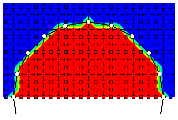
Finally, a quick note about mesh generation. Right now, Starfish supports just the “staircase” method. The code simply uses the provided surface boundary to figure out which mesh nodes are internal, and these nodes are given the boundary condition of the surface spline. A more detailed method of using cut cells is still in development. You can see in Figure 2 below the staircasing effect. Zooming in on the circle, we can see which nodes are flagged as internal (red contour) and which are external (blue). The Poisson solver smoothes out these irregularities, but the solution will be slightly different than if the geometry was correctly resolved. Implementing cut cells or a similar approach remains as future work.

Continue to Starfish Tutorial Part 2.

Starfish Tutorial Part 1: Domain, Boundaries, and a Potential Solver