Modeling Diffuse Reflection (or How to Sample Cosine Distribution)

Molecules impacting surfaces may reflect either specularly or diffusely, depending on surface properties. The diffuse reflection is by far more common and hence it’s important that it’s implemented in the code correctly. In a diffuse interaction, the molecule actually temporarily attaches to the target. The time spent on the surface is known as residence time, and it will be tiny for surfaces at temperatures above the molecule condensation temperature. In this process, the molecule completely “forgets” its original direction and leaves the surface in a new random direction. But there is one important caveat: flux of outgoing molecules is proportional to the cosine from the surface normal. This is known as Lambert’s cosine law. Sampling from this cosine distribution is the topic of this article.
Incorrect Way
Before I show you the correct way to model diffuse reflection, I wanted to talk a bit about the incorrect way. The reason I am mentioning this is that on first sight, this incorrect way actually seems acceptable. In fact, it is what was being used in my plume simulation code Draco for a while. Oops! But first, a bit of geometry.
Computationally, we define a planar surface element (be it a triangle, a quad, or so on) with three local unit vectors: a surface normal, and two tangents. The actual orientation of the tangents is not important since we are sampling random orientation. The important characteristic is that \(\mathbf{n}=\mathbf{t}_{1}\times\mathbf{t}_{2}\). The obvious algorithm for sampling diffuse reflections then may seem to be to select a random multiplier for each of the three unit vectors, add the resulting components together, and convert to a unit vector. Since we are sampling only in the positive half-space of the surface normal (assuming normal pointing outward), the algorithm is as follows (remember, this is incorrect!):
#pick three random numbers
a = -1 + 2*random()
b = -1 + 2*random()
c = random()

#multiply by corresponding directions
v1 = [a*n for n in tang1]
v2 = [b*n for n in tang2]
v3 = [c*n for n in norm]

#add up to get velocity, vel=v1+v2+v3
vel = []
for i in range(0,3):
    vel.append(v1[i]+v2[i]+v3[i])

#make a unit vector
vel_mag = math.sqrt(vel[0]*vel[0]+vel[1]*vel[1]+vel[2]*vel[2])
for i in range(0,3):
   vel[i] /= vel_mag
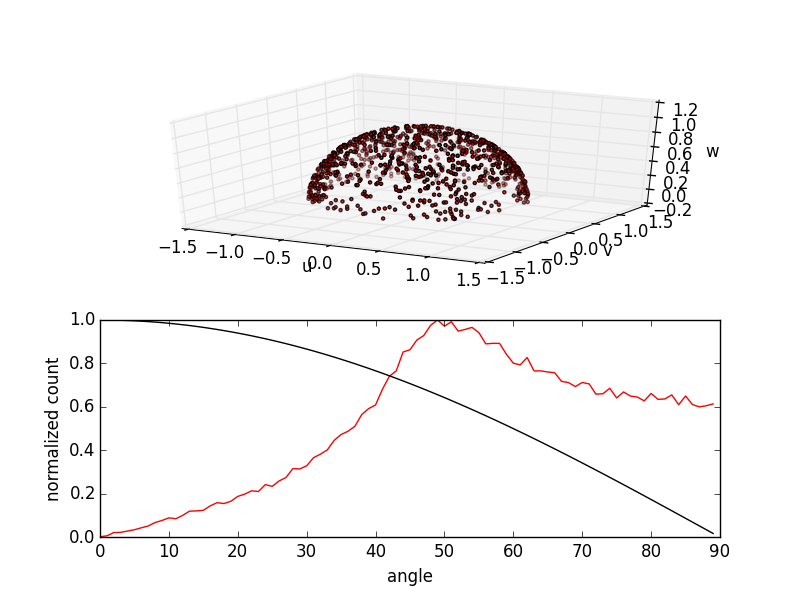
The full code is listed in random3.py, available at the link below. Now, if we do this for a large number of particles, and for each compute the cosine from the surface normal, we will obtain an angular distribution as shown below. As we can see, the resulting distribution is not right. Majority of particles bounce off at angles closer to 50 degrees, instead of the expected zero.
Sampling from Cosine Distribution
Instead, in order to model diffuse reflections correctly, we need to perform two steps:
- Sample component along the normal, \(\mathbf{v}_|\), from the cosine distribution
- Rotate the perpendicular component \(\mathbf{v}_\perp\) about a random \(0:2\pi\) angle
This is given by the following set of equations:
$$\begin{align}
\sin \theta &= \sqrt{\mathcal{R}_1}\\
\cos \theta &= \sqrt{1-\sin^2\theta}\\
\psi &= 2\pi\mathcal{R}_2\\
\mathbf{v}_1 &= \cos\theta \mathbf{n}\\
\mathbf{v}_2 &= \sin\theta \cos\psi\mathbf{t}_1\\
\mathbf{v}_3 &= \sin\theta \sin\psi\mathbf{t}_2\\
\mathbf{v} &= \mathbf{v}_1+\mathbf{v}_2+\mathbf{v}_3
\end{align}
$$
where \(\mathcal{R}\) are two random numbers in the range of [0:1). The computation of cosine comes from the identity that \(\cos^2\theta + \sin^2\theta = 1\).
Numerically, this is written as follows:
sin_theta = math.sqrt(random())
cos_theta = math.sqrt(1-sin_theta*sin_theta)

#random in plane angle
psi = random()*2*math.pi;

#three vector components
a = sin_theta*math.cos(psi)
b = sin_theta*math.sin(psi)
c = cos_theta

#multiply by corresponding directions
v1 = [a*n for n in tang1]
v2 = [b*n for n in tang2]
v3 = [c*n for n in norm]

#add up to get velocity, vel=v1+v2+v3
vel = []
for i in range(0,3):
    vel.append(v1[i]+v2[i]+v3[i])
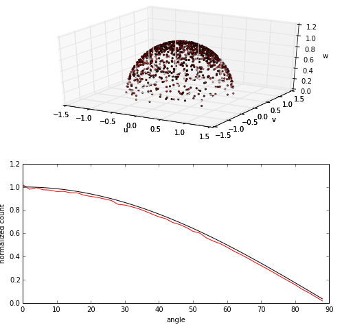
If we again plot a histogram of the angular distributions, we will obtain a trace as shown below in Figure 2. A much better agreement is seen!
Why sample from sine?
If you look at the code closely, you will notice that we are actually picking a random number that corresponds to the sine of theta, not the cosine. Is this a mistake?
No, it’s not. The reason the sampling works this way is that in order to sample from an arbitrary distribution, you actually need to sample from the cumulative distribution function (CDF) of the probability density function. This is known as the inverse transform method, and you will find more info in the references [1], [2], and [3], noted below. But in short, the CDF tells you the probability of finding some value (x) in the range \(-\infty:x\). In other words, it is the sum of the probabilities up to the value point. Numerically it is written as
$$F_X(x) = \int_{-\infty}^x f_x(\xi) d\xi$$
The importance of CDF is that it ranges from 0 at the left boundary to 1 at the right boundary, which is also what we get from the random number generator. In the case of a periodic function like cosine, we have
$$\begin{align}
F_{cos}(\theta) &= \int_{0}^\theta \cos(\xi) d\xi\\
&=\sin(\theta) – \sin(0)\\
&=\sin(\theta)
\end{align}
$$
Source Code
You can download the two example Python scripts below. Also, I recently started adding the blog examples to Github. You may be interested in cloning the following repo: github.com/particleincell/PICCBlog.
random3.py (illustrates the incorrect way)
cosine.py (correct sampling for diffuse reflection)
Refrences
[1] Generating Random Variates
[2] Lecture 3: Inverse Transform Method
[2] Sampling via Inversion of the cdf
What’s the reasoning behind the sqrt in:
sin_theta = math.sqrt(random())
There is a paper by John Greenwood that goes into the derivations: The correct and incorrect generation of a cosine distribution of scattered particles for Monte-Carlo modelling of vacuum systems. Basically, and you can try this yourself by running the Python code, you want to generate cosine distribution per surface area. Without the square root, you will get cosine distribution per angle. This will however result in an incorrect flux, that is highly focused around the normal direction.
I guess if x is uniform in [0, 1] then also sqrt(x) is uniform in [0, 1], but it only seems to be an unnecessary computation?
Lubos, thanks for the link. I found this (and reading up on the inverse transform method) to be helpful in understanding the derivations.
Another question though: In your Python code example, you calculate the area of each “bin” using the formula:
A = 2 * pi * ((1-cos(t2)) - (1-cos(t1)))
Could you explain this a bit more? Is this taking Lambert’s cosine factor into account, or is it just plain geometry? Any clarification would help, thanks.
Thank you for this post. I was pulling my hair out assuming particles left a surface in completely random directions.
What sort of surfaces reflect specularly? Also, how does that affect the desorption of particles?
Not sure – I generally use diffuse reflection for all surface impacts.
Thanks Lubos;
I know most surfaces reflect light specularly. Do you know of any that reflect gas particles specularly? Perhaps it depends on surface preparation?
I spoke to some colleagues about this and it seems that in general molecules reflect diffusely. However, there may be some cases of high speed molecules impacting cryogenic surfaces that result in specular-like reflections: https://www.princeton.edu/~gscoles/theses/sean/chapter2.html
Hi,
I’m doing a simulation of particles in a box in 2D, and instead of reflection for the collisions on the wall I would like to use the cosine law.
so for example when a particle hit the upper wall for the reflection case :
if position[j][0] – radius<edgeY:
v[j][1]=-1*(v[j][1])#Vy reflected
position[j]=[radius+edgeY+2,position[j][1],0]
but now if I want to use cosine law:
sin_theta = math.sqrt(random.random())
cos_theta = math.sqrt(1-sin_theta*sin_theta)
#random in plane angle
psi = random.random()*2*math.pi;
v[j][0]=math.sqrt(v[j][0]*v[j][0]+v[j][1]*v[j][1])*sin_theta #Vx
v[j][1]=math.sqrt(v[j][0]*v[j][0]+v[j][1]*v[j][1])*cos_theta #Vy
With that I thought I would end up with a distribution equivalent to the cosine distribution with phi=0, i.e a quarter of a circle. But I ends up with a probability of reflection around 50 degrees.
Do you have any idea why ?
Anyway thank you for this very cool website.