Two Stream Instability Javascript Simulation

On this page you will find my first cut at simulating two-stream instability using Javascript with PIC (recently I also added a Vlasov version). You can also load the demo in full window. The simulation will start automatically in 5 seconds. You can also start and pause it using the first button. The second button resets the particle population. You will need to use this in order for the settings, except the ones on the “Solver” line, to take place.
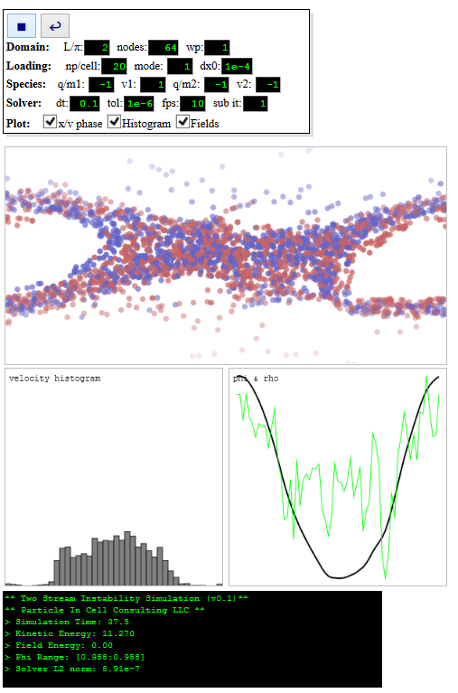
Screenshot
Below is a screen shot of what the simulation should look like:
About the simulation
Two stream instability is a well-known problem in plasma physics. It was studied extensively by Birdsall in his classic Plasma Physics via Computer Simulation. The simulation consists of two beams, infinitely large in y and z direction (so you have a 1D problem) streaming through each other. In the standard setup, the charge to mass ratio of the two beams is identical. The velocity magnitudes are also equal, but the velocities have opposite direction. This system is unstable, and any small perturbation grows until the streaming is destroyed. Some particles get trapped in vortices in the position-velocity phase space. Other particles on the other speed up to about 3x their initial velocity.
When writing this code, I tried to replicate Birdsall’s setup from his ES1 program as much as possible. However, one big difference is the potential solver. ES1 uses Fast Fourier Transform to solve the Poisson’s equation in the periodic space. This is the correct approach, but as I didn’t have an FFT code quite ready at my disposal, I implemented the solver using the Gauss-Seidel with Successive Over Relaxation Technique. I envision that in the future version I’ll replace this with the FFT. As such, the results I am getting are not completely equal to what Birdsall shows in his book. It’s possible there is a mistake/difference somewhere else as well. Please leave a comment if you find some issues!
Simulation Inputs
Here is a summary of the inputs. Values in parentheses are the defaults.
L/π: Domain length will be this parameter multiplied by π (2)
nodes: Number of mesh nodes (64)
wp: Plasma frequency, used to compute charge (1)
np/cell: Number of particles per cell (20)
mode: Perturbation mode (1)
dx0: Perturbation magnitude (1e-4)
q/m1: Charge over mass for species 1 (-1)
v1: Drift velocity of species 1 (1)
q/m2: Charge over mass for species 2 (-1)
v2: Drift velocity of species 2 (-1)
tol: Poisson solver tolerance (1e-6)
dt: Time step (0.1)
fps: Animation frames per second (10)
sub it: Simulations steps between animations (1)
You may notice that some of these values don’t look physical. That’s because the simulation runs with ε0 (permittivity of free space) set to 1. The particle charge is computed from plasma frequency as
$$q = \omega_p^2 \left(\frac{1}{q/m}\right) \epsilon_0 \frac{L}{N};$$
where \(N\) is the number of particles per species. Particles are loaded offset from a uniformly distributed center, \(x_i =x_{0,i} + \hat{x}_{i}\), where \(x_{0,i}=(i+0.5)\Delta x\) and \(\hat{x}_{i} = \Delta x_0 \cos(2\pi\cdot\text{mode}\cdot x_{0,i}/L)\)
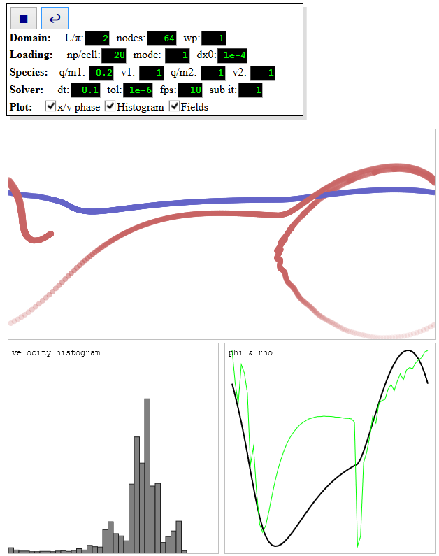
Suggestions
Feel free to play with these inputs. What happens if one of the streams is much more massive than the other one? Or what if the velocities are not equal in magnitude? What is the impact of mode and domain length on the simulation?
Implementation
Two-stream instability simulation is a great project for introduction to the PIC method. In fact, I remember this being one of our projects in the Plasma Simulation course I took at Virginia Tech by Prof. Wang (I also remember struggling to get it working!). Please see my older post on the ES-PIC method for some of the details. But you should find the code quite straightforward. You can by the way download the entire code by right clicking on the attachment below.
Particle Loading
Particles are loaded using the following script:
/*new empty list*/
$.parts = [];

/*uniform seeding*/
var delta_x = $.L/np;

/*disturbance data*/
var mode=getVal("mode",1);
$.dx0 = getVal("dx0",0.0001);

for (var p=0;p<np;p++)
{
	var x0 = (p+0.5)*delta_x;

	/*perturb positions*/
	var theta = 2*Math.PI*mode*x0/$.L;
	var dx = $.dx0*Math.cos(theta);
	var x1 = x0+dx
	var x2 = x0-dx;

	if (x1<0) x1+=$.L;
	if (x2<0) x2+=$.L;
	if (x1>=$.L) x1-=$.L;
	if (x2>=$.L) x2-=$.L;

	$.parts.push(new Part(x1,vmag1,0,q1,m1));
	$.parts.push(new Part(x2,vmag2,1,q2,m2));
}
Particle In Cell (PIC) Iteration
The main PIC simulation iteration is given by the following code
/*clear rho*/
for (var i=0;i<ni;i++)
	rho[i] = 0;

/*scatter particles to grid*/
for (var p=0;p<np;p++)
{
	/*get particle logical coordinate*/
	var lc = $.parts[p].x/dh;
	var i = Math.floor(lc);
	var q = $.parts[p].q;
	var d = lc-i;
	rho[i]+=q*(1-d);
	rho[i+1]+=q*d;
}

/*add stationary background charges,
ni-1 because last and first node are the same*/
for (var i=0;i<ni-1;i++)
	rho[i] += $.q0*(np/(ni-1));

/*apply periodic bc*/
rho[ni-1] += rho[0];
rho[0] = rho[ni-1];

/*divide by cell size to get charge density*/
for (var i=0;i<ni;i++)
	rho[i] /= dh;

/*remove noise*/
for (var i=0;i<ni;i++) if (Math.abs(rho[i])<1e-10) rho[i]=0;

/*solve potential*/
phi[0]=0;
for (var i=0;i<ni;i++) phi[i]=0;
for (var solver_it=0;solver_it<20000;solver_it++)
{
	for (var i=0;i<ni-1;i++)
	{
		var im = i-1; if (im<0) im=ni-2;
		var ip = i+1;if (ip==ni-1) ip=0;
		var g = 0.5*((rho[i]/$.EPS0)*dh*dh + phi[im] + phi[ip]);
		phi[i] = phi[i]+1.4*(g-phi[i]);
	}

	/*convergence check*/
	if (solver_it%25==0)
	{
		var sum=0;
		for (var i=1;i<ni-1;i++)
		{
			var ip = i+1;if (ip==ni-1) ip=0;
			var res=rho[i]/$.EPS0+(phi[i-1]-2*phi[i]+phi[ip])/(dh*dh)
			sum += res*res;
		}
		$.l2 = Math.sqrt(sum/ni);
		if ($.l2<tol) break;

	}
}
phi[ni-1]=phi[0];

/*electric field*/
for (var i=0;i<ni;i++)
{
	var im = i-1;
	var ip = i+1;
	if (im<0) im=ni-2;
	if (ip>ni-1) ip=1;

	ef[i] = (phi[im]-phi[ip])/(2*dh);
}

/*update positions*/
for (var p=0;p<np;p++)
{
	var P = $.parts[p];

	/*interpolate EF to particle position*/
	var lc = $.parts[p].x/dh;
	var i = Math.floor(lc);
	var d = lc-i;
	var ef_p = ef[i]*(1-d) + ef[i+1]*d;

	/*first time rewind velocity 0.5dt*/
	if (it==0) P.v -= 0.5*ef_p*P.qm*dt;

	/*update velocity*/
	P.v += ef_p*P.qm*dt;

	/*update position*/
	P.x += P.v*dt;

	/*periodic boundary for particles*/
	if (P.x<0) P.x += $.L;
	if (P.x>=$.L) P.x -= $.L;
}
Code
two-stream.html: Download the code by right clicking and choosing “Save as”. You will also find the code on Github.
Please leave a comment if you enjoyed this simulation and/or found a bug (or it just doesn’t work at all on your system!). Also, remember that developing interactive HTML5 codes such as this one is something that we specialize at Particle In Cell Consulting LLC. Please send us an email for a quote.
Also, I’ll be shortly adding option to resize the graph windows.
Dear Sir,
are there any codes written in matlab for this simulation?
it is really interesting and glad that you share it to everyone
thank you
Its amazing what you can do with Java script sir 🙂
Cool!!!
Thanks Daoru! I was trying to find my code written for Joe’s class back in 2002 but only found the submitted homework. See you guys in Japan?
Very interesting … Have you tried programming for Android devices ?
Hi Raed, not yet. I bought an Android programming book while back but haven’t spent much time on it. However I agree, this could be a neat demo. Although in theory the code should work as is on an Android phone from the web browser. It at least works on my iphone.
Nice Job!
I am a iOS developer and also a Ph.D from Space Science, I am trying to do the same work by using swift and metal. Just want to see the performance when running on iOS device.
Keep me posted Tim. I can add a link once you get it working. What university are you at?
Hello Sir,
Is there any way to implement the same in c++?
Sure, of course. But I don’t have the C++ version but will gladly look over yours (or can post it here) if you send it to me.
Great animation, has been very helpful in getting to grips with the instability.
I’m currently trying to match the dynamics seen here with my own finite difference PIC code, but haven’t been able to figure how to do periodic boundary conditions for Poisson’s equation in finite difference.
Do you have any advice sir?
Kristoffer – implementing periodic boundaries is quite simple. You just treat the “left” and “right” nodes as the same. So, on the left most node you have “phi[-1]-2*phi[0]+phi[1]”. However, since the right most node phi[ni-1] is the same as phi[0], this is identical to “phi[ni-2]-2*phi[0]+phi[1]”