Potential Solver for Composite Dielectrics

In a previous post, we discussed how to solve the non-linear Poisson’s equation frequently encountered in plasma simulations, where the non-linearity came from an analytical model for electron density. The solver however treated only the free charge in “vacuum” due to the presence of electrons and ions. In this post, we’ll see how to compute the electric potential across a mixed medium consisting of pieces of a varying electric permittivity.
Governing Equations
We start by defining the displacement field [1],
$$\mathbf{D} = \epsilon_0 \mathbf{E}+ \mathbf{P}$$
where \(\mathbf{E}\) and \(\mathbf{P}\) are the electric and polarization density fields, respectively. The polarization term captures the field due to “trapped” dipole moments in the material matrix. Taking a divergence of both sides, we obtain \(\nabla\cdot\mathbf{D} = \epsilon_0 \nabla\cdot\mathbf{E}+ \nabla\cdot\mathbf{P}\) or
$$\epsilon_0 \nabla\cdot\mathbf{E} = \nabla\cdot\mathbf{D} – \nabla\cdot\mathbf{P}$$
Comparing this to Gauss’ law, \(\epsilon_0 \nabla\cdot\mathbf{E} = \rho\), we see that
$$ \rho = \nabla \cdot \mathbf{D} – \nabla \cdot \mathbf{P} \equiv \rho_f + \rho_b$$
In other words, charge density can be decomposed into components due to “free” and “bound” charges, given by \(\rho_f=\nabla \cdot \mathbf{D}\) and \(\rho_b = -\nabla \cdot \mathbf{P}\). If the material is linear (polarization is directly proportional to the applied field), homogeneous (there is no spatial variation), isotropic (there is no directional variation), the polarization density field can be written in terms of the electric field as \(\mathbf{P} = \epsilon_0 \chi \mathbf{E}\), where \(\chi\) is the electric susceptibility. With this definition, we obtain
$$ \mathbf{D} \equiv \epsilon_0 (1+\chi) \mathbf{E} = \epsilon_0 \epsilon_r \mathbf{E} = \epsilon \mathbf{E}$$
where \(\epsilon_r\) is a non-dimensinal “relative permittivity”, and \(\epsilon\) is the material’s permittivity in F/m. Again taking divergence of both sides and using our definition of the free charge density, we obtain the following version of Gauss’ law,
$$\nabla \cdot \mathbf{D} \equiv \nabla \cdot (\epsilon \mathbf{E}) \equiv \epsilon\nabla\mathbf{E}+ \mathbf{E}\nabla \epsilon= \rho_f \qquad \qquad (1)$$
where the free charge density is the contribution from electrons and ions we encounter in our plasma simulations. We can also see that if there is no variation in permittivity, and if we are dealing only with charges in free space, we recover the original form, \(\epsilon_0 \nabla \cdot \mathbf{E} = \rho\).
Introducing Electric Potential
We next discuss how to compute the electric potential, and indirectly the electric field, in composite materials with a varying permittivity. This allows us to model the effects of dielectrics, materials with a limited ability to conduct electric field by polarization. We can in fact see from the previous equation that “permittivity” is inversely related to the electric field. The higher the permittivity, the smaller the change in electric field due to the same free charge density, \(\nabla \cdot \mathbf{E} = \rho_f / (\epsilon_0 \epsilon_r)\). Permittivity thus seems as a pretty poor choice for the name. With the model we develop below, we will be able to set fixed Dirichlet boundaries by specifying regions with an artificially high permittivity.
Helmholtz decomposition (a.k.a. the fundamental theorem of vector calculus) tells us that any vector field can be split into a a sum of irrotational (zero curl) and solenoidal (zero divergence) components, \(\mathbf{F}= -\nabla \phi + \nabla \times \mathbf{A}\). From Faraday’s Law, we see that if there is no temporal variation in magnetic field, the electric field is irrotational,
$$\nabla \times \mathbf{E} = – \dfrac{\partial \mathbf{B}}{\partial t}\equiv 0$$
This is known as the electrostatic approximation. With this in mind, we rewrite the Gauss’ law (Equation 1) in terms of the electric potential,
$$\epsilon \nabla \phi + \nabla \phi \nabla \epsilon = -\rho_f \qquad \qquad (2)$$
This is the equation that we need to solve. We will assume that our domain consists of multiple materials, each having its own permittivity. This then results in the two following observations:
- There is no variation in permittivity within a piece, and thus Equation 2 reduces to \(\epsilon\nabla^2\phi = -\rho_f\). This is the standard form of the Poisson’s equation we have been solving in the past. For a 1D Cartesian mesh, the discretization is given by \(\epsilon(\phi_{i-1} -2\phi_i + \phi_{i+1}) = -\rho_{f,i}\Delta^2 x \).
- There is a discontinuity in permittivity across the interface. We address this in the next section.
Interface Boundary
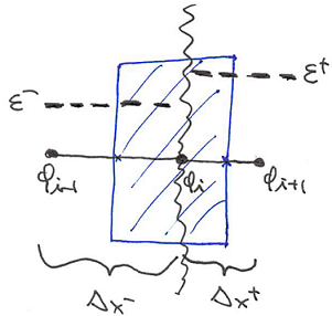
Defining a control volume centered on the interface, Figure 1, we use the divergence theorem to rewrite \( \nabla \cdot (\epsilon \nabla \phi)=-\rho_f \) as
$$ \oint_S{\epsilon \nabla \phi \cdot \mathbf{n} \text{d}A }= -\rho_f \Delta V$$
Following the finite volume method, we assume any variation in the tangential direction is negligible, leaving us with
$$ (\epsilon \nabla_x \phi )^+ – (\epsilon \nabla_x \phi)^-= -\rho_f \Delta x \equiv -\sigma_f$$
where \(\sigma_f\) is the surface charge. Allowing for a variable mesh spacing between pieces, the above equation can be discretized as
$$ \frac{\epsilon^-(\phi_i – \phi_{i-1})}{\Delta x^-} – \frac{\epsilon^+(\phi_{i+1} – \phi_i)}{\Delta x^+} = \rho_f \left(\frac{\Delta x^+ + \Delta x^-}{2}\right)$$
or
$$ \phi_i = \left[\rho_f \left(\frac{\Delta x^- + \Delta x^+}{2}\right)(\Delta x^+ \Delta x^-) + \epsilon^-\Delta x^+ \phi_{i-1} + \epsilon^+\Delta x^- \phi_{i+1}\right] \left(\frac{1}{\epsilon^-\Delta x^+ + \epsilon^+\Delta x^-}\right) \qquad (3)$$
where we assumed that the interface is at the \(i\)th node.
Numerical Implementation
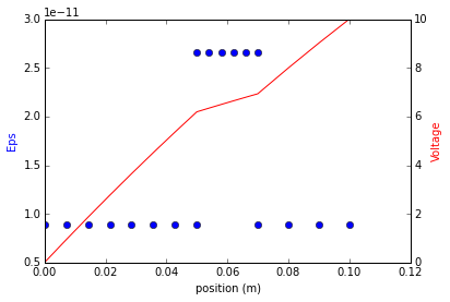
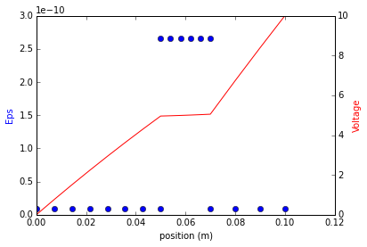
The above algorithm was implemented in Python. You can download the source code here. When you run it, you will get an output similar to Figure 2. This figure compares the effect of relative permittivity (commonly also known as dielectric constant) on the solution. We can see that as it is increased, the potential becomes more constant. It also starts approaching the initial value that was set on these nodes (zero in our case). In the limit of \(\epsilon \to \infty, \phi\to\phi_0\).
Code starts by defining the pieces. The parameter list specifies the length of the piece, number of nodes, and the relative permittivity.
#define pieces
pieces = []
pieces.append(Piece(0.05,8,1));
pieces.append(Piece(0.02,6,3));
pieces.append(Piece(0.03,4,1));
We next initialize the potential field and the charge density. The left and right boundaries are fixed (Dirichlet nodes), and the potential is initialized to zero. This is important, since the potential will tend to drive towards this initial value on pieces with high permittivity.
#boundaries
phi_bc = (0,10)

#initial potential array
phi = [0]*nn
phi[0] = phi_bc[0]
phi[nn-1] = phi_bc[1]

#charge density
rho_f = [2e10*Q]*nn
Below is the actual solver. The solver simply performs 1000 Gauss Seidel iterations without doing any convergence checking.
#solver loop
for it in range(1,1000):
    #iterate over pieces
    for k in range(0,len(pieces)):
        p = pieces[k]
        #set left node per interface b.c. except for first piece
        if (k>0):
            eps_plus = p.eps
            eps_minus= pieces[k-1].eps
            dh_plus = p.dh
            dh_minus = pieces[k-1].dh
            i = p.offset
            sigma_f = rho_f[i]*0.5*(dh_plus+dh_minus)
            phi[i] = 1.0/(dh_minus*eps_plus+dh_plus*eps_minus)*(sigma_f*dh_plus*dh_minus + \
                        eps_plus*dh_minus*phi[i+1] + eps_minus*dh_plus*phi[i-1])

        #on piece-internal nodes, solve poisson's equation nabla^2 phi = -rho/eps
        for i in range(p.offset+1,p.offset+p.nodes-1):
            if (i<nn-1):
                phi[i] = 0.5*(phi[i-1]+phi[i+1]+rho_f[i]/p.eps*p.dh*p.dh)
Source Code
References
[1] Jackson, J.D., Classical Electrodynamics, Wiley & Sons, 3rd ed., 1999