Quasi Steady-State Testing Approach for High Power Hall Thrusters

In the late 2021, I, along with Drs. Yevgeny Raitses, Edgar Choueiri, Roger Myers, and Prof. Michael Keidar published a paper in Journal of Applied Physics special issue on electric propulsion on a concept of testing high-power Hall thrusters using a pulse operation (doi:10.1063/5.0067232). This work involved performing numerical simulations with a modified version of HPHall that allows for a background density build up due to a limited pumping speed. It also allows for a cyclic operation in which the thruster is mass flow rate is varied between the nominal and the low mode. While it is not possible to publicly share the HPHall source code modifications or the result files, I wanted to share here the scripts that were generated to process the data.
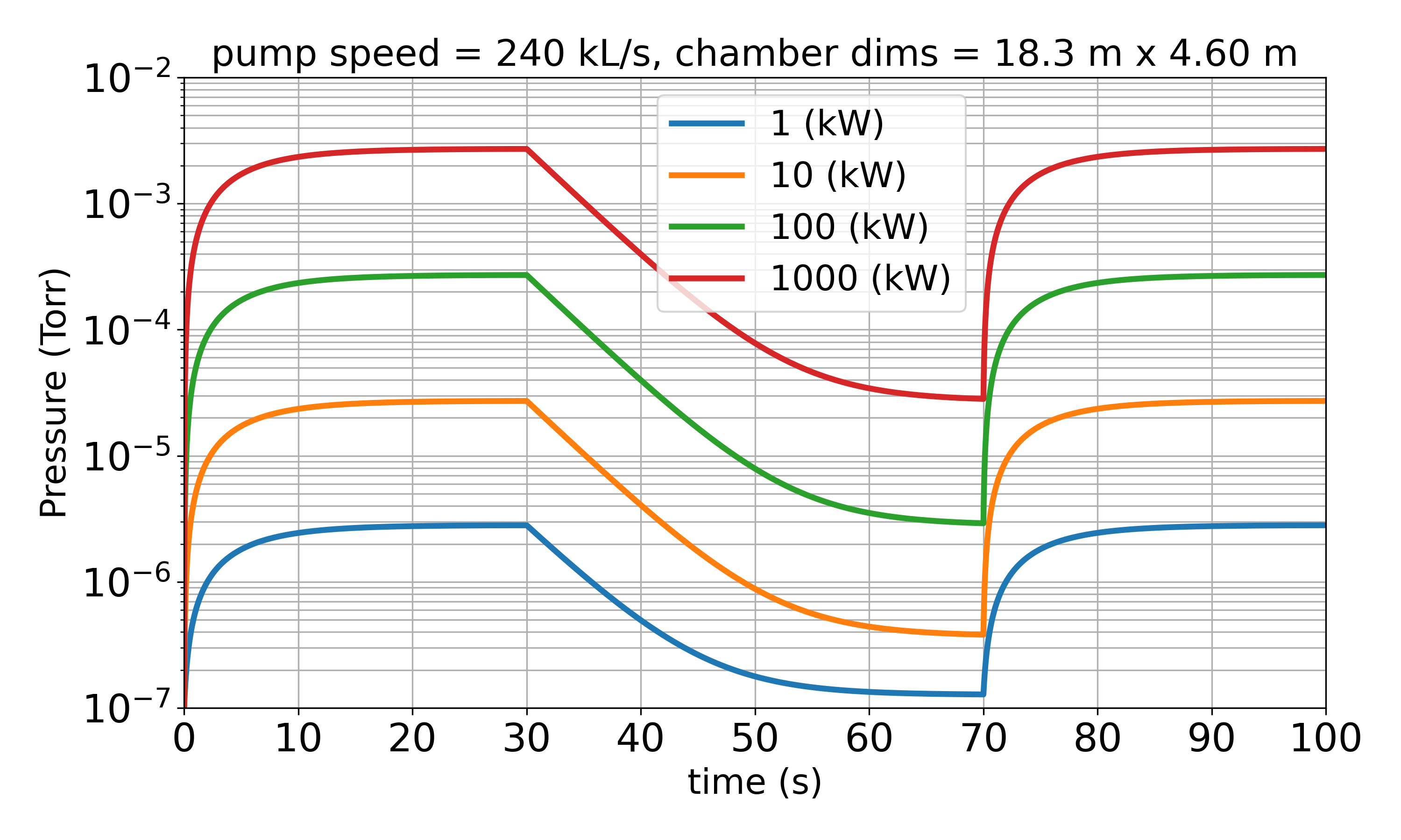
First, a simply Python program was developed to estimate the pressure in a vacuum chamber given some thruster power and pumping speed. This code, pump.py, assumes the chamber is a 0D volume and does not consider any transit time or pressure non-uniformities. It was used to generate plots like
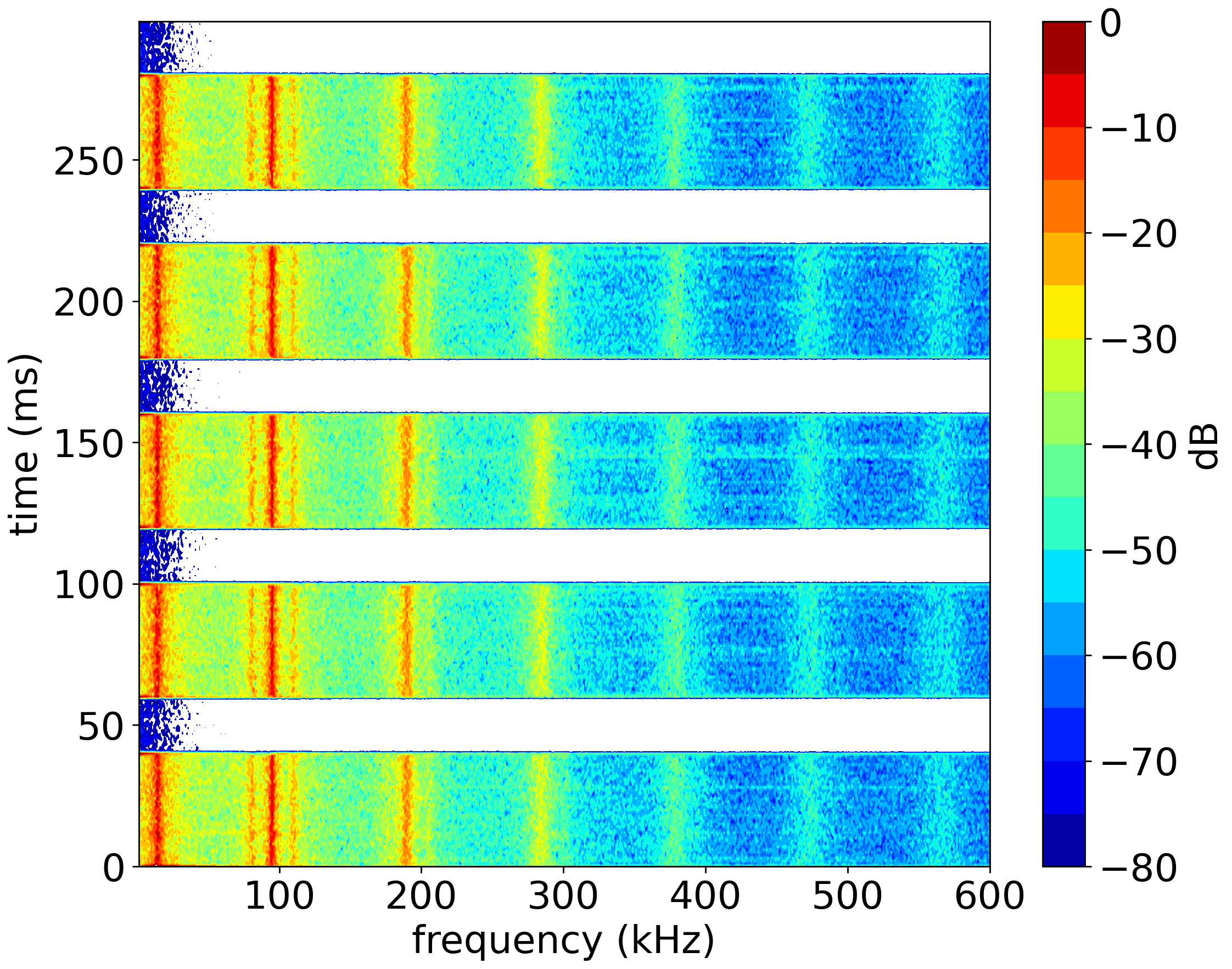
The second program, frequency_series.py, reads in HPHall log.csv and pulls out the time varying discharge current, as well as thrust. The primary purpose of the script is to use a moving window coupled with Python’s FFT subroutines to create a “waterfall” spectogram of the discharge current evolution. It can be used to generate plots like shown in Figure 2.
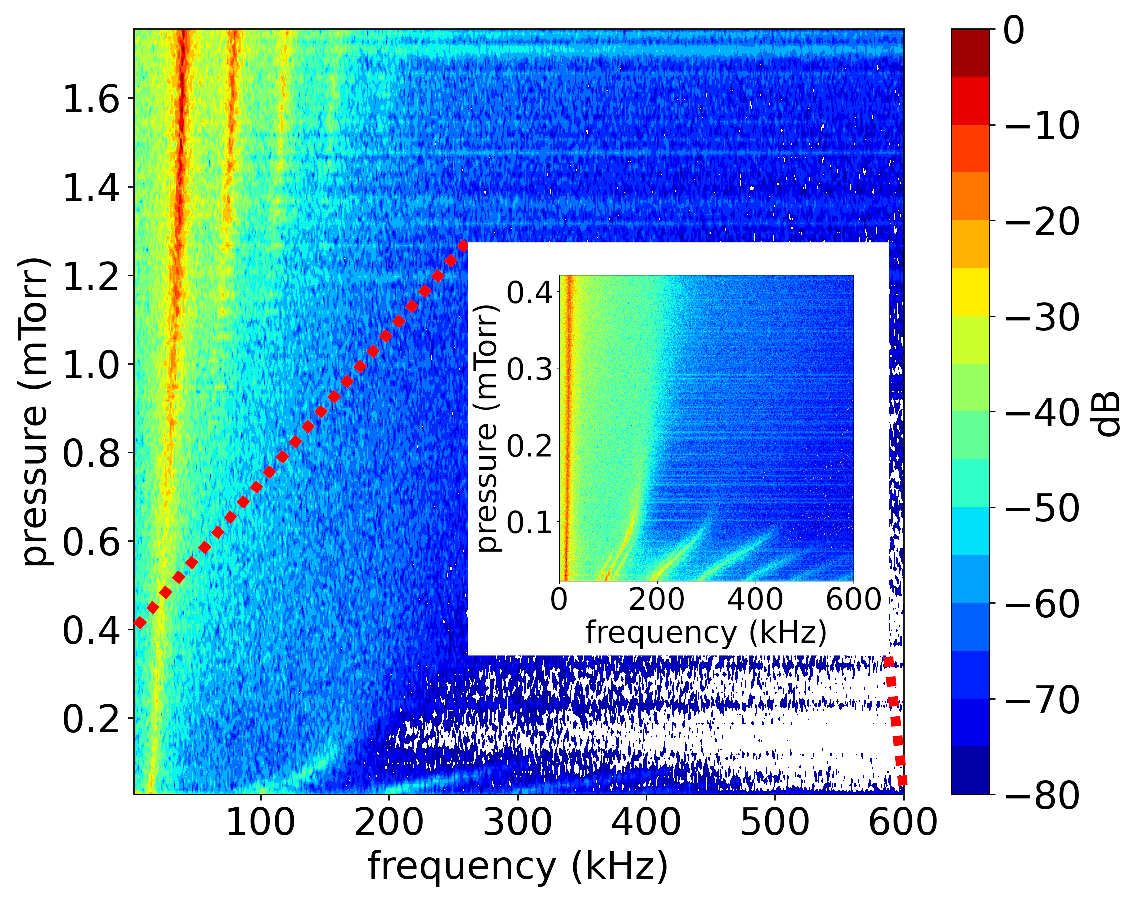
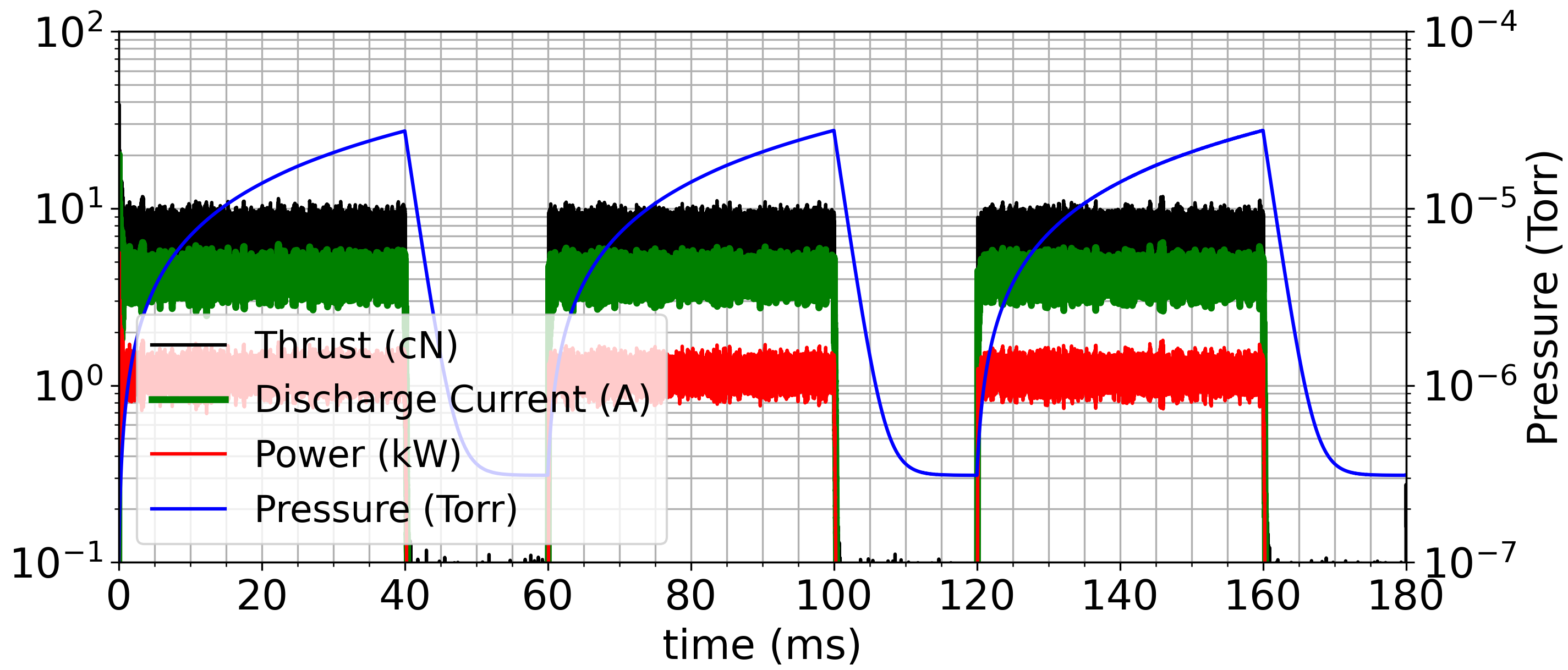
The thruster operating parameters are also visualized as shown in Figure 3.
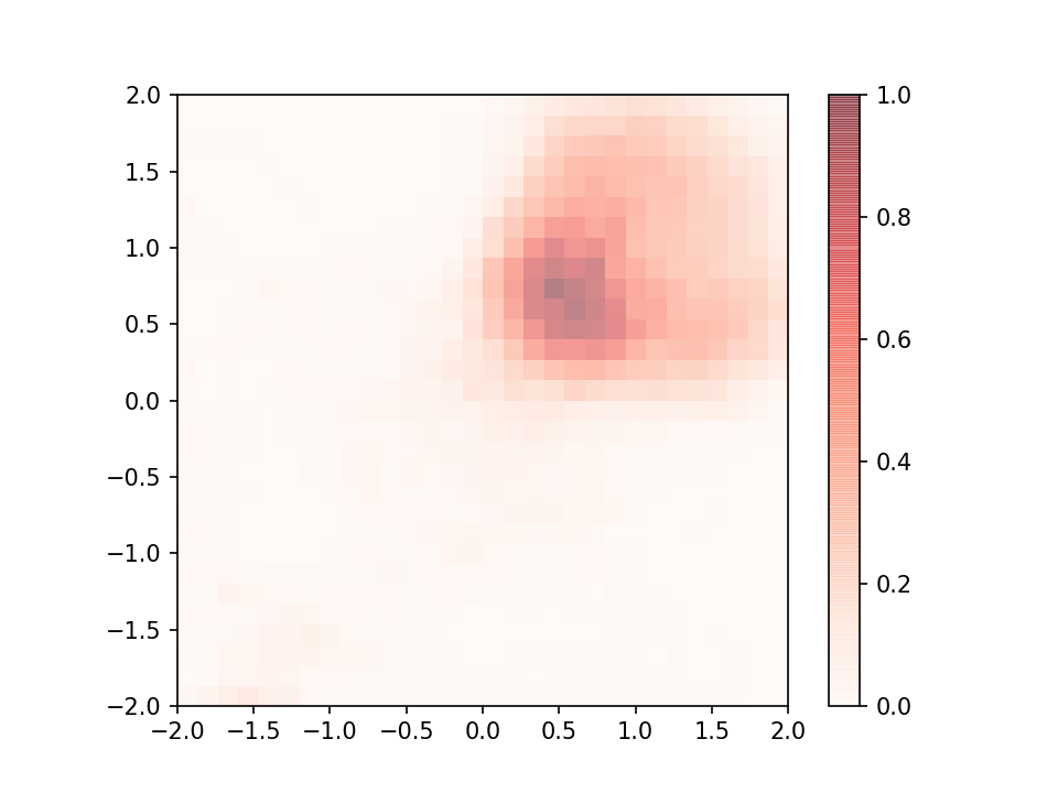
This program can also be optionally (disabled by default) used to generate a time-lag phase portrait. These plots are however not shown in the paper as I couldn’t really get anything useful out of them. The idea behind these portraits is that they allow us to compare two different signals in a way that preserves phase information, which is otherwise lost in an FFT. You simply trace out a curve formed by \(f(t)\) and \(f(t-\tau)\) as the \(x\) and \(y\) points. The plot in Figure 4 is the heat map of this curve. A perfectly harmonic signal will just trace out a circle or an ellipse, depending on the selection of \(\tau\).