HTML5 + Javascript DSMC Simulation

Posted on December 26th, 2012
Previous Article :: Next Article

The Demo

In the previous article we presented a crash-course in the Direct Simulation Monte Carlo (DSMC) method (DSMC is an algorithm for simulating gas flows using computational macroparticles instead of fluid equations as is the case with CFD, Computational Fluid Dynamics). The article also contained an interactive example that demonstrated DSMC by colliding two populations in a single simulation cell. We will now go through the steps of getting this example working. You’ll find the demo right here:

Source Code

First, make sure to download the source code: dsmc0.html (right click and select “save as”)

Modern web browsers are truly powerful tools that allow you to do some amazing things, like run a mesh generator, or show interactive plots. This particular demo relies on three technologies: HTML5 for the page markup and the canvas element, CSS3 to add fancy style with shadows, and Javascript to perform the actual simulation and generate the animated plot. Long gone are days when Javascript was slow! The demo shown here runs 500 time steps with 2000 particles and had to be artificially slowed down to see the evolution in the velocity distribution function.

HTML / CSS3

Starting with the HTML markup, here is the entire source code in a nutshell:

<!-- Javascript+HTML DSMC Demo, Lubos Brieda, Dec 2012
Please visit https://www.particleincell.com/2012/html5-dsmc for more info -->
 
<canvas id="cell" style="border:1px solid #888;box-shadow:10px 10px 5px #888;" width=600 height=400>
<h2>Your browser does not support the &lt;canvas&gt; element. Please use a different browser or 
click <a href="https://www.particleincell.com/2012/dsmc0/">here</a> if you are viewing this in an email.</h2>
</canvas>
 
<script> 	
/* --- JAVA SCRIPT HERE --- */
</script>
 
<form action="" style="padding-top: 20px">
<input type="button" value="Start the simulation!" style="font-size:1.2em;color:green;" onclick="startSim();">
</form>

Before we get started, notice that the file is not a fully-enclosed HTML document. In other words, it does not have the <html> and <body> tags. This is to allow inserting this snippet into the blog post. If you are developing a stand-alone web-application, you will want to make sure to include these elements as well.

The source code begins with a short notice which serves mainly as a pointer back to this page, in case you forgot where you got the source code from. Next, a canvas element is created. Canvas is one of the several additions in HTML5. You should not have any problem seeing the canvas unless you have a truly archaic browser. One exception however is email. Even modern browsers will not render canvas in email messages. Many people read this blog via the newsletter and as such, we want to include a link for them to click on to display the page outside of the email reader. We also set the dimensions and apply styling to the canvas. The styling consists of 1 pixel thick solid gray border complimented by a drop shadow. In the past, you had to utilize various “*-kit” alternatives to get the shadow working, but this no longer seems to be necessary.

The code ends with a simple form used merely to add a button which starts the simulation. The button is given some styling and we also attach an event handler to it. In between is bunch of Javascript which we will get into later. This Javascript is quite important – without it, your browser would render the following:

canvas with shadow — Figure 1. This is what you would see without any Javascript

Canvas manipulation with Javascript

Here is a part of the Javascript code:

/*grab canvas and related properties*/
var canvas=document.getElementById("cell");
var ctx = canvas.getContext("2d");
var height=canvas.height;
var width=canvas.width;
 
/*paint background before we scale the context*/
var grad=ctx.createRadialGradient(0,0,width/200,0,0,width/2);
grad.addColorStop(0,"purple");
grad.addColorStop(1,"rgba(255,255,255,0)");
ctx.fillStyle=grad;
ctx.fillRect(0,0,width,height);
 
/*create axis*/
ctx.strokeStyle="black";
ctx.fillStyle="purple";
ctx.lineWidth=3;
setLineDashSafe([10,6]);
ctx.strokeRect(0.05*width,0.05*height,0.9*width,0.9*height);
setLineDashSafe([]);
 
/*save background*/
var saved_bk = ctx.getImageData(1, 1, width, height);
 
/*scale to [0,1][0,1] and put origin at left/bottom to simplify graphing*/
ctx.translate(0.05*width,0.95*height);
ctx.scale(0.9*width,-0.9*height);
 
/*show initial distribution*/
dsmcCell.init();
 
/*helper function since Firefox does not seem to support setLineDash*/
function setLineDashSafe(style)
{
    if (ctx.setLineDash)
        ctx.setLineDash(style);
}

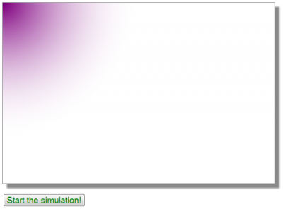
To get things rolling, we first add a bit of color to the canvas to make it more visually appealing. We start by grabbing the canvas element and its 2D context. The drawing is actually done not by the canvas but by the context. We also grab the canvas dimensions. We then create a radial gradient transitioning from opaque purple to transparent white. This gradient is centered at point (0,0) which initially happens to be the top-left corner. The radial gradient is specified by providing positions and radii of two circles, here the two dimensions are 1/200th and 1/2 of the width. We fill the entire canvas with this gradient. This gives us the following:

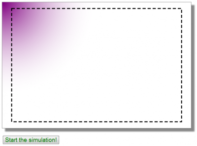
canvas with radial gradient — Figure 2. Initial canvas filled with a radial gradient

We next create the axis. I got lazy, and instead of painting the x and y axis with tick marks and the appropriate labels, I decided to plot just a dashed rectangle indicating the axis extends. During the testing, I found out that Firefox does not seem to support the setLineDash canvas property and hence I am using a wrapper that sets the dash only if this function is defined. Otherwise the code would crash due to an uncaught extension (I could have also wrapped this call in the try clause). After we plot the rectangle, the canvas should look like this:

canvas with gradient and dashed rectangle — Figure 3. Final background with a dashed axis border

We are now done drawing the background. The main difference between the canvas element and SVG (as for instance demonstrated in the Bezier splines article) is that the canvas element is a stateless bitmap. In SVG, we can add and remove elements as needed. But to do an animations with the canvas, we need to repaint the entire frame. Instead of filling the background and replotting the rectangle at each time step, it is much more efficient to save the generated background bitmap. This is done with the

var saved_bk = ctx.getImageData(1, 1, width, height);

command. We will later repaint the background using

/*restore background*/
ctx.putImageData(saved_bk, 1, 1);

Finally, the initial canvas dimensions range from (0,0) in the top right corner to (600,400) in the bottom right. When dealing with XY plots, it may be more natural for the y-axis to go from the bottom to the top. It is also more natural to think of coordinates as ranging from 0 to 1. This scaling is done with

/*scale to [0,1][0,1] and put origin at left/bottom to simplify graphing*/
ctx.translate(0.05*width,0.95*height);
ctx.scale(0.9*width,-0.9*height);

The translate shifts the origin (0,0) to the bottom left corner of the dashed rectangle. The coordinate (1,1) corresponds to the top right corner. The flip over the y-axis is done by scaling the y-direction by a negative number. Also, please note that this scaling is done after we finished drawing the dashed rectangle. The scaling affects everything, not just the position. Namely, it would affect the shape of the gradient as well as the spacing between dashes. Since our canvas is not a square, we would end up with different dash spacing on the horizontal and vertical faces had we applied the transformation earlier. Finally, we call the DSMC init function. This function is described below.

The XY plot

The actual velocity distribution function is plotted using the following code:

/*generates XY plot from xy[2][]*/  
function plotXY(xy)
{
   var x=xy[0],y=xy[1];
 
   /*restore background*/
   ctx.putImageData(saved_bk, 1, 1);
 
   /*start plotting*/
   ctx.beginPath();
   ctx.moveTo(0,0);
   for (var i=0;i<x.length;i++)
       ctx.lineTo(x[i],y[i]);
 
    /*return to the first point, and fill*/
    ctx.lineTo(1,0);
    ctx.lineTo(0,0);
    ctx.fill();
}

This function takes in as an argument a 2D array in the form xy[2][], with both components assumed to range from 0 to 1. For convenience, this array is split into two 1D arrays. The function then repaints the background using the previously saved bitmap. We then use the beginPath command to start plotting a linear trace. We move to the origin, and then create a bunch of linear segments to all (x,y) tuples from the input data set. At the end, we add a line to the bottom right corner and then back to the origin to create a closed polygon. This polygon is then filled with the fill style, which happens to be purple.

Javascript DSMC Code

We are now ready to tackle the meat of the project: the actual DSMC simulation. The entire DSMC code is encompassed within a Javascript “class”:

/***** START OF DSMC CLASS *****/
var dsmcCell = (function() {
var AMU = 1.66053886e-27;	/*atomic mass*/
var K = 1.3806488e-23;		/*Boltzmann constant*/
var V_c=0.001*0.01*0.001;	/*cell volume*/
var sigma_cr_max=1e-18;		/*initial guess*/
var Fn = 5e8;			/*macroparticle weight*/
 
var delta_t=2e-5;		/*time step length*/
var it;				/*current iteration*/
var vdf;			/*public array to hold VDF data*/
 
var part_list = new Array(); /*particle list*/
 
/*particle class, creates particle with isotropic velocity*/	
function Part(vdrift,temp,mass)
{
 /**** CODE BELOW ****/
}
 
/*creates initial particle populations*/
function init()
{
 /**** CODE BELOW ****/
}
 
/* performs a single iteration of DSMC*/	
function performDSMC()
{
 /**** CODE BELOW ****/
}
 
/*samples from 1D Maxwellian using the Birdsall method*/
function maxw1D()
{
 /**** CODE BELOW ****/
}
 
/*returns random thermal velocity*/
function sampleVth(temp,mass)
{
 /**** CODE BELOW ****/
}
 
/*evaluates cross-section using a simple inverse relationship*/
function evalSigma(rel_g) 
{
 /**** CODE BELOW ****/	
}
 
/*returns magnitude of a 3 component vector*/
function mag(v)
{
 /**** CODE BELOW ****/
}
 
/*performs momentum transfer collision between two particles*/
function collide (part1, part2)
{
 /**** CODE BELOW ****/
}
 
/* bins velocities into nbins between min and max */
function computeVDF(min, max, nbins)
{
 /**** CODE BELOW ****/
}
 
/*expose public members*/	
return {init:init,performDSMC:performDSMC,vdf:vdf};
})();
/**** END OF DSMC CLASS *****/

Although Javascript does not include a direct “class” counterpart to Java or C++, you can define analogous functionality using Javascript functions. What’s important to notice is that only the objects included in the return statement at the end of the code will actually be public – and thus exposed to the rest of the code. The rest of the variables and functions are private to the class. This is true with the variables we define at the beginning. These include some constants, as well as an array that will be used to hold the particles.

Particle class

We use an inner class to represent each particle. This code is given below:

function Part(vdrift,temp,mass)
{
	this.v=[];
 
	/*sample speed*/
	var vth = sampleVth(temp,mass);
 
	/*pick a random direction*/
	var theta = 2*Math.PI*Math.random();
	var R = -1.0+2*Math.random();
	var a = Math.sqrt(1-R*R);
 
	this.v[0] = vth*Math.cos(theta)*a;
	this.v[1] = vth*Math.sin(theta)*a;
	this.v[2] = vth*R + vdrift;
 
	this.mass=mass;
}
 
/*samples from 1D Maxwellian using the Birdsall method*/
function maxw1D()
{
	return 0.5*(Math.random()+Math.random()+Math.random()-1.5);		
}
 
/*returns random thermal velocity*/
function sampleVth(temp,mass)
{
	var sum=0;
	var vth = Math.sqrt(2*K*temp/mass);
	for (var i=0;i<3;i++)
	{
		var  m1 = vth*maxw1D();
		sum += m1*m1;
	}
 
	return Math.sqrt(sum);
}

The “constructor” takes as inputs drift velocity, gas temperature, and particle mass, and creates a random particle with an isotropic velocity sampled from the Maxwellian at the corresponding thermal velocity. The this.* construct is used to create inner members that hold the particle velocity and mass. Here we use two helper functions to sample the 3D Maxwellian distribution.

DSMC Init function

The particles are loaded by the init function:

/*creates initial particle populations*/
function init()
{
	/*clear data, important if restarting*/
	part_list = [];
	it = 0;
 
	/*first create slow particles*/
	for (var i=0;i<1000;i++)
		part_list.push(new Part(100,5,32*AMU));
 
	/*and now the fast ones*/
	for (var i=0;i<1000;i++)
		part_list.push(new Part(300,5,32*AMU));
 
	/*show initial plot*/
	vdf = computeVDF(0,450,25);
	plotXY(vdf);
}

The first step here is to clear the list. This is important since we give the user the ability to run the simulation repeatedly. Without this step, the particle list would grow with each click of the “Start Simulation” button! We create two populations, each consisting of 1000 particles. In a real DSMC simulation, you would have a much fewer particles per cell – likely no more than 100 total. However, here we use the higher number to obtain a smoother VDF plot. The particles come in two populations, one with drift velocity of 100 m/s and the other having drift velocity 300 m/s. Both are given initial temperature of 5K to generate a tight beam. This is quite cold, since for the relatively light molecular mass considered here, higher thermal velocities would exceed the drift speed.

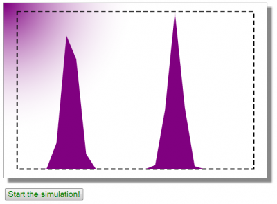
In a more involved example, we could get these parameters from a user form, but here for simplicity, they are hardcoded. But feel free to experiment with changing these values on your end. You may also want to change the ratio in particle counts between the two populations, this will influence the final average velocity. At the end of this function, we make a call to compute the VDF and to plot it. This will give us the initial view the user will see until he or she presses the “Start Simulation” button, which is plotted below in Figure 5.

canvas with xy plot — Figure 4. The initial view showing the two initial populations

Pressing the button fires the following code:

/*handler for the button click*/
function startSim()
{
	dsmcCell.init();
	dsmcCell.performDSMC();
}

We first make a call to the init function. This is not needed the first time, in fact, we cheat here a bit in that the populations that will be collided will be slightly different than what the user sees on screen when the page is loaded the first timie. This could be avoided by, for instance, calling init only if the time step (it) is greater than zero – meaning the code had run previously. But for simplicity, this is not done here. We then call performDSMC, which performs a single step of the DSMC method.

NTC DSMC method

The code is shown below. It implements Bird’s DSMC NTC method.

/* performs a single iteration of DSMC*/	
function performDSMC()
{
	/*fetch number of particles*/
	var np = part_list.length;
 
	/*compute number of groups according to NTC*/
	var ng_f = 0.5*np*np*Fn*sigma_cr_max*delta_t/V_c;
	var ng = Math.floor(ng_f+0.5);	/*number of groups, round*/
	var nc = 0;			/*number of collisions*/
 
	/*for updating sigma_cr_maxx*/
	var sigma_cr_max_temp = 0;
	var cr_vec = [];
 
	/*iterate over groups*/
	for (var i=0;i<ng;i++)
	{
		var part1,part2;
 
		/*select first particle*/
		part1=part_list[Math.floor(Math.random()*np)];
 
		/*select the second one, making sure the two particles are unique*/
		do {part2=part_list[Math.floor(Math.random()*np)];}
		while (part1==part2);
 
		/*relative velocity*/
		for (var j=0;j<3;j++)
			cr_vec[j] = part1.v[j]-part2.v[j];		
		var cr = mag(cr_vec);
 
		/*eval cross section*/
		var sigma = evalSigma(cr);
 
		/*eval sigma_cr*/
		var sigma_cr=sigma*cr;
 
		/*update sigma_cr_max*/
		if (sigma_cr>sigma_cr_max_temp)
			sigma_cr_max_temp=sigma_cr;
 
		/*eval prob*/
		var P=sigma_cr/sigma_cr_max;
 
		/*did the collision occur?*/
		if (P>Math.random())
		{
			nc++;
			collide(part1,part2);
		}
	}
 
	/*update sigma_cr_max if we had collisions*/
	if (nc)
		sigma_cr_max = sigma_cr_max_temp;
 
	/*show diagnostics*/
	vdf = computeVDF(0,450,25);
	plotXY(vdf);
 
	it++;
 
	/*output more data to the console*/
	console.log("it: "+it+"tng: "+ng+"tnc: "+nc+"tscmax: "+sigma_cr_max);
 
	/*run for 500 time steps*/
	if (it<500)
		setTimeout(performDSMC,10);
}
 
/*evaluates cross-section using a simple (non-physical) inverse relationship*/
function evalSigma(rel_g) 
{
	return 1e-18*Math.pow(rel_g,-0.5);
}
 
/*returns magnitude of a 3 component vector*/
function mag(v)
{
	return Math.sqrt(v[0]*v[0]+v[1]*v[1]+v[2]*v[2]);
}

We first estimate the number of collision groups, and then perform that many collision checks. For each check, we select at random two particles, making sure they are unique. We then compute the relative velocity and obtain the cross-section using a simple inverse model. Note: this cross-section model was selected at random and is not supposed to be physically sound! The collision probability is then compared to a random number, and if the collision occurred, we call the collision handler.

Elastic collision handler

The collision handler is given below. It implements an elastic collision between two particles with isotropic scattering angle.

/*performs momentum transfer collision between two particles*/
function collide (part1, part2)
{
	/*center of mass velocity*/
	var cm = [];
	for (var i=0;i<3;i++)
		cm[i] = (part1.mass*part1.v[i] + part2.mass*part2.v[i])/
			(part1.mass+part2.mass);
 
	/*relative velocity, magnitude remains constant through the collision*/
	var cr=[];
	for (var i=0;i<3;i++)
		cr[i] = part1.v[i]-part2.v[i];
 
	var cr_mag = mag(cr);
 
	/*pick two random angles, per Bird's VHS method*/
	var theta = Math.acos(2*Math.random()-1);
	var phi = 2*Math.PI*Math.random();
 
	/*perform rotation*/
	cr[0] = cr_mag*Math.cos(theta);
	cr[1] = cr_mag*Math.sin(theta)*Math.cos(phi);
	cr[2] = cr_mag*Math.sin(theta)*Math.sin(phi);
 
	/*post collision velocities*/
	for (var i=0;i<3;i++)
	{
		part1.v[i] = cm[i]+part2.mass/(part1.mass+part2.mass)*cr[i];
		part2.v[i] = cm[i]-part1.mass/(part1.mass+part2.mass)*cr[i];	
	}		
}

The math for this handler is taken from Bird. We first compute the center of mass velocity, as well as the magnitude of the relative velocity (note, this could be passed in to optimize the code). We then sample two angles per Chapter 11 in Bird. These two angles are used to rotate the relative velocity into a new coordinate frame. Finally, the velocities of the two particles are adjusted. As an aside, this model implements isotropic scattering. However, in reality, non-isotropic scattering models tend to be more accurate descriptions of what happens in molecular collisions, especially in the field of plasma ion momentum transfer collisions. Hence in a real simulation, you would want to select the theta angle from the differential cross-section.

Diagnostics

All that’s needed now is to bin the particle data into a histogram that can be plotted with our plotXY function. This is done via the following function:

/* bins velocities into nbins between min and max */
function computeVDF(min, max, nbins)
{
	/*pointers for easier access*/
	vel = [];
	bin = [];
 
	/*set delta range*/
	var delta = (max-min)/(nbins-1);
 
	/*shift left by half delta to center bins*/
	min -= 0.5*delta;
	max -= 0.5*delta;
 
	/*set initial values*/
	for (var i=0;i<nbins;i++) 
	{
		vel[i] = i/(nbins-1);
		bin[i] = 0;
	}
 
	/*compute histogram*/
	for (var i=0;i<part_list.length;i++)
	{
		var part = part_list[i];
		var vmag = mag(part.v);
		var b = Math.floor((vmag-min)/(delta));
		if (b<0 || b>=nbins-1) continue;
		bin[b]++;
	}
 
	/*normalize values*/
	var max_bin=0;
	for (var b=0;b<nbins;b++) 
		if (bin[b]>max_bin) max_bin=bin[b];
 
	for (var b=0;b<nbins;b++)
		bin[b]/=max_bin;
 
	return [vel, bin];
}

This function returns a 2D array consisting of “velocity” and the “bin” count. Both fields are actually normalized. The velocity array is assigned linearly increasing values in the range of 0 to 1. The bin counts are also divided by the maximum bin count, also yielding data in the range of 0 to 1. This normalization is done to simplify the visualization.

In addition, we also output data to the console in the performDSMC function. This is done using the following code:

console.log("it: "+it+"tng: "+ng+"tnc: "+nc+"tscmax: "+sigma_cr_max);

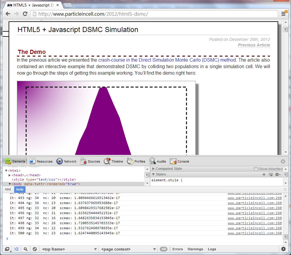
The console is normally hidden, but you will find it under “inspect element” right click menu in Chrome, or “Developer Tools” in Internet Explorer. The console will show you the number of groups, number of collisions, and the sigma_cr_maax parameter determined for each time step.

chrome console diag output — Figure 5. The console showing some additional diagnostic output

Animations with HTML5 Canvas and Javascript

We are now almost done. All that’s needed is the animation part. This is actually quite simple. At the end of each time step, the performDSMC function makes a call to plotXY to show the updated VDF. This code is repeated below:

vdf = computeVDF(0,450,25);
plotXY(vdf);
 
it++;
 
/*run for 500 time steps*/
if (it<500)
	setTimeout(performDSMC,10);

After the plot is made, the simulation time step is incremented. As long as the time step is less than 500 (the maximum number of time steps), the function then adds a timeout to call itself again in 10 milliseconds.

And that’s all. Feel free to leave a comment if you have any questions or something is not clear.

See More Interactive Demos

For more interactive demos, make sure to check out the SVG mesh generator, write up on smooth Bezier splines, and the article on HMTL5 plotting.