Loading an isotropic velocity distribution

Particle methods such as the Particle In Cell Method (PIC) or Direct Simulation Monte Carlo (DSMC) simulate a gas discharge by advancing particles through small steps until some final steady state is reached. But how do we actually get the particles into the simulation in the first place? This article deals with this very important topic, known as particle loading.

The velocity with which particles are born essentially specifies one of the simulation initial conditions. The PIC / DSMC methods simply model the evolution of this initial distribution. Hence, it is crucial that the initial distribution accurately represents the physical situation. Regardless how accurate your solver is, you can’t expect anything but garbage if you feed the solver garbage inputs. Our simulation codes such as Starfish or CTSP allow the user to load particles from both surface and volume sources using a wide range of velocity distribution models. Surface sources are used to model gas injection. These sources inject particles in the direction of the surface normal according to a prescribed distribution. The simplest example would be a uniform beam that simply injects particles with the same velocity and direction. A more realistic model is a drifting Maxwellian. In this source, the particle velocity varies according to the temperature of the gas – the hotter the gas, the greater the variation. The Maxwellian distribution is also used to load background species – those of you with a physics background will right away know that this distribution describes the distribution of velocities in a thermalized gas (one that has undergone a sufficient number of collisions).

Method 1 (Incorrect)

Here we consider the simplest form of a volume source, a source that injects particles with uniform speed and a uniformly-distributed velocity direction. If such a source is a point source, it can be imagined to be a infinitely small light source, with light beams emitting uniformly in all directions. Hence at time 0 we will have only an infinitely small point. At some later time t1 the leading front of the particles will describe the surface of a sphere. The sphere will get bigger as the time goes on, with the density decreasing accordingly.

So how do we inject such particles? First let’s consider the most obvious, but incorrect approach.

/*pick random direction*/
n[0] = -1.0 + 2*Math.random();
n[1] = -1.0 + 2*Math.random();
n[2] = -1.0 + 2*Math.random();
 
/*normalize to a unit vector*/
double n_mag = Math.sqrt(n[0]*n[0] + n[1]*n[1] + n[2]*n[2]);
n[0] /= n_mag;
n[1] /= n_mag;
n[2] /= n_mag;
 
/*assign velocity*/		
part.v[0] = n[0]*v_mag;
part.v[1] = n[1]*v_mag;
part.v[2] = n[2]*v_mag;

This code picks a random direction along each axis, scales the vector to unity, and multiplies it by the velocity magnitude. Simple, but incorrect. If you run this code for a while, you will get a density contour such as the one shown in Figure 1 (the example code for this example is provided in the post on particle data structures). We were expecting a sphere, but instead the particles are expanding as a cube.

Method 2 (Isotropic Direction)

The reason why the first method doesn’t work is that it is actually behaving correctly, however, the algorithm is incorrect. Think about what a random number generator does. Its goal is to uniformly fill the space between the lower and the upper limit ([0:1) for the normalized case). In 1D, a random number generator will uniformly fill a line. In 2D, it will uniformly fill a square. And in 3D, it will fill a cube, which is exactly what we saw.

Instead, we need to get a bit more clever. We can divide the problem into two steps. First, let’s consider the x-y plane. We can obtain a uniform circular distribution by first selecting a random angle, and then using trigonometry to obtain the x and y coordinates. In other words, \(\theta=[0:2\pi)\), \(n_x=\cos(\theta)\) and \(n_y=\sin(\theta)\). This loading is shown below in Figure 2.

/*pick a random angle*/
double theta = 2*Math.PI*Math.random();
 
/*compute vector*/
n[0] = Math.cos(theta);
n[1] = Math.sin(theta);
n[2] = 0;

Almost there, we just need to add the third direction. Let’s think about what we want to accomplish. We want the vector to be uniformly distributed along the z axis. At the same time, we want to assure that the vector has a unit magnitude. This will require scaling the x-y component by some factor a. Hence we write \(n_z = [-1:1]\), \(n_x=a\cos(\theta)\) and \(n_y=a\sin(\theta)\). We need \(n_x^2+n_y^2+n_z^2=1\), or \(a^2\cos^2(\theta)+a^2\sin^2(\theta)+n_z^2=1\). This gives us \(a=\sqrt{1-n_z^2}\) by the trig identity. We modify our example code accordingly,

/*pick a random angle*/
double theta = 2*Math.PI*Math.random();
 
/*pick a random direction for n[2]*/
double R = -1.0+2*Math.random();
double a = Math.sqrt(1-R*R);
 
n[0] = Math.cos(theta)*a;
n[1] = Math.sin(theta)*a;
n[2] = R;

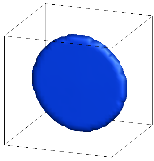
and voila, we get the right distribution, as shown in Figure 3! As a little aside, the implementation here has a little bug. Java’s Math.random returns values in the range of [0:1) (zero inclusive but one exclusive). Hence, there will be a slight preferential minus z direction, since \(n_z=[-1:1)\). This could be corrected by using a modified RNG that is one-inclusive.