Particulate Contamination Transport on Orbiting Satellites

Lately I’ve been working on simulating transport of particulate contaminants on an orbiting satellite. I am not going to get into the results but wanted to at least summarize the approach as I thought this was an interesting problem. And since my background in orbital mechanics is quite limited, this way I also hope to bring in a wider audience. Don’t hesitate to chime in if the method is totally bogus!

So what’s the issue? Spacecraft thermal surfaces are often painted with black or white paint, depending on the desired thermal properties. Paints can “particulate”, or shed small, dust-like particles. This process may arise from acoustic loads during launch, or from deployment of appendages on orbit. The question is: if particulates are released, what fraction of them comes back to contaminate the satellite?

Now, we know that in absence of forces, particles will move in a straight line and only impact surfaces within their line of sight. But, once forces are considered, the answer is less clear. But what forces act on particulates in space? First, aerodynamic drag can be neglected due to low pressure, especially for geostationary satellites. There are also electrostatic forces as particles can charge up. But if we assume that charge over mass remains small, these forces should also be negligible. There is however one more force that needs to be considered: gravity. You may be thinking, these dust flakes are very tiny, and the force of gravity will also be small. That may be the case, but what we are specifically talking about is the force of gravity affecting orbital bodies.

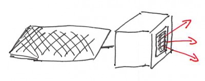
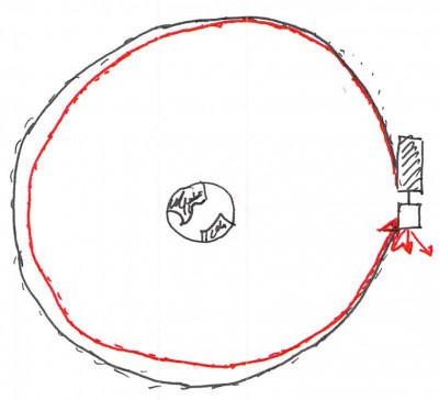
Take a look at the sketch in Figure 1. The bottom face of the spacecraft bus is a source of particulates. Even though there are no surfaces within a direct line of sight, we may end up with particulate contamination on the spacecraft once orbital motion is considered. Why is this? Well, in Keplerian orbital mechanics, there is a one-to-one relationship between position along an orbit and the orbital velocity. This means that if a particle is launched at some point \(\vec{x}_0\) with velocity offset from the parent body \(\Delta \vec{v}_0\ne \vec{0}\), then this particle will necessarily fall onto a different orbit from the parent object. Furthermore, in the absence of drag or perturbations (more on this below), the two orbits will again intersect at this point. Now, the period of the new orbit will be different from the parent body. But, as long as the initial delta velocity is small enough, the temporal difference between the two crossings will be small, and the dust flake will impact the satellite. This is basically the gist of what I attempted to model.

Gravitational Force

The force acting on all orbiting bodies is given by Newton’s Law of Universal Gravitation,
$$\vec{F}_G = -\frac{GMm}{r^2} \frac{\vec{r}}{r}$$
In this formulation, \(\vec{F}_G\) is the force acting on a body with mass \(m\) by the body with mass \(M\). Vector \(\vec{r}\) is \(\vec{r}_2-\vec{r}_1\) and \(r=|\vec{r}|\). The gravitational constant \(G=6.674\times 10^{-11}\) Nm² kg^-2. Once the force is computed, the incremental velocity is computed from
$$\Delta\vec{v}_G=\frac{\vec{F}}{m}\Delta t$$
and the position can be integrated using the standard Leapfrog integrator (care must be taken to use small enough time steps).

Python Implementation

I used Python to test out the algorith before implemeting it in CTSP. The code (newton.py) is listed below.

# -*- coding: utf-8 -*-
"""
Demo of particulate contaminant transport on an orbiting satellite, solar drag not considered
 
Created on Mon Jan 11 10:13:01 2016
https://www.particleincell.com/2016/particulate-orbit/
@author: lbrieda
"""
 
import numpy as np
import pylab as pl
 
def mag(a):
    return np.sqrt(np.dot(a,a))
 
Ra=42164e3   #Ra is the initial apoapsis radius
Rp=1*Ra      #Rp is the initial periapsis radius
G= 6.67408e-11 #gravitational constant
Me=5.972e24
GM = G*Me  #GM=3.98e14  #G*M for earth
 
v0 = 3070
dt=60     #dt is the time-step for numerical solution
num_it=20000
 
#init
pos=np.zeros((num_it,3))
pos[0]=np.array([Rp,0,0]);
vel=np.zeros((num_it,3))
vel[0]=np.array([0,v0,0])
 
vel_dust = np.zeros_like(vel);
pos_dust = np.zeros_like(pos);
pos_dust[0,:] = pos[0,:]
vel_dust[0,:] = vel[0,:]
dp = [0,0,0]
dv = [-0.05,0,0]
pos_dust[0] += dp;
vel_dust[0] += dv;
#vel_dust[0] += np.append(200*(1-2*np.random.random(2)),0)
 
#rewind
r = pos[0]
r_mag = mag(r)
a=-GM*r/(r_mag**3)
vel[0] -= 0.5*a*dt
 
r = pos_dust[0]
r_mag = mag(r)
a=-GM*r/(r_mag**3)
vel_dust[0] -= 0.5*a*dt
 
for it in range(1,num_it):
    #r-vector, earth is at (0,0,0)
    r = pos[it-1]
    r_mag = mag(r)
    a=-GM*r/(r_mag**3)
    vel[it] = vel[it-1]+a*dt
    pos[it] = pos[it-1]+vel[it]*dt
 
    #dust
    r = pos_dust[it-1]
    r_mag = mag(r)
    a=-GM*r/(r_mag**3)
    vel_dust[it] = vel_dust[it-1]+a*dt
    pos_dust[it] = pos_dust[it-1]+vel_dust[it]*dt
 
#load CTSP results    
#ctsp_sat = np.loadtxt("cg_pos.txt")
#ctsp_part = np.loadtxt("part_pos.txt")
 
fig = pl.figure(figsize=(18,8))
ax = fig.add_subplot(121)
ax.plot(pos[:,0],pos[:,1],'k')#marker='o',markersize=4);      # plot initial orbit
ax.hold(True);
ax.plot(pos_dust[:,0],pos_dust[:,1],'b');             # plot initial orbit
#add CTSP orbit
#ax.plot(ctsp_sat[:,0],ctsp_sat[:,1],'k:',linewidth="2",marker='o',markersize=4,markevery=100);
#ax.plot(ctsp_part[:,3],ctsp_part[:,4],'b:',linewidth="2",marker='o',markersize=4,markevery=100);
pl.legend(['Python sat','Python dust','CTSP sat','CTSP dust'])
pl.title('Orbits for dv=(%.2f,%.2f,%.2f)'%(dv[0],dv[1],dv[2]))
pl.axis("equal")
 
ax = fig.add_subplot(122)
d=pos_dust-pos
ax.plot(d[:,0],d[:,1],'r-');             # plot initial orbit
ax.hold(True);
#ax.plot(ctsp_part[:,0],ctsp_part[:,1],'r:',linewidth="2",marker='o',markersize=4,markevery=10);
pl.legend(['Python','CTSP'])
pl.title('Relative position of dust')
pl.savefig("plot.png",dpi=180,format="PNG",pad_inches=0.0,bbox_inches="tight")

This code includes several commented out lines that were used to verify the implementation in CTSP (when it comes to V&V of simulation codes, verification checks that equations are implemented correctly, while validation checks that the correct equations are implemented). Getting the code working in CTSP required performing transformations between local and earth inertial coordinate frames hence the need for this verification. Results with large injection delta velocity are shown below in Figure 2. Each of the four sets of images shows the orbit of the satellite (black) and dust (blue) on left. In this figure, Earth is at (0,0). The second set shows the relative position between the satellite and the particulate. Here (0,0) indicates collision. In both sets of plots, solid lines are results from the Python simulation and dotted lines with markers correspond to data loaded from CTSP. You won’t have this second set of data when running the demo code. The two lie on top of each which is what I wanted to see.

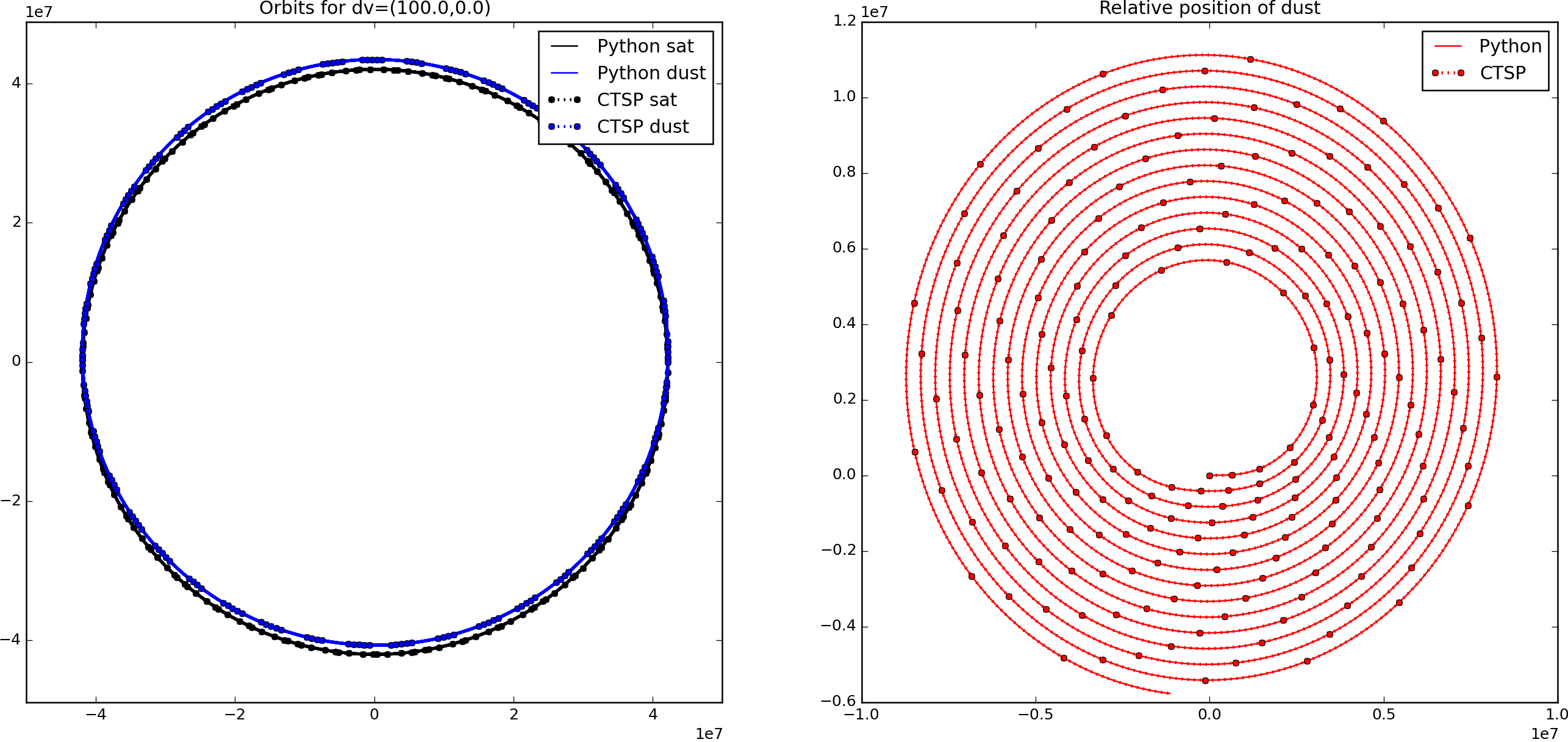
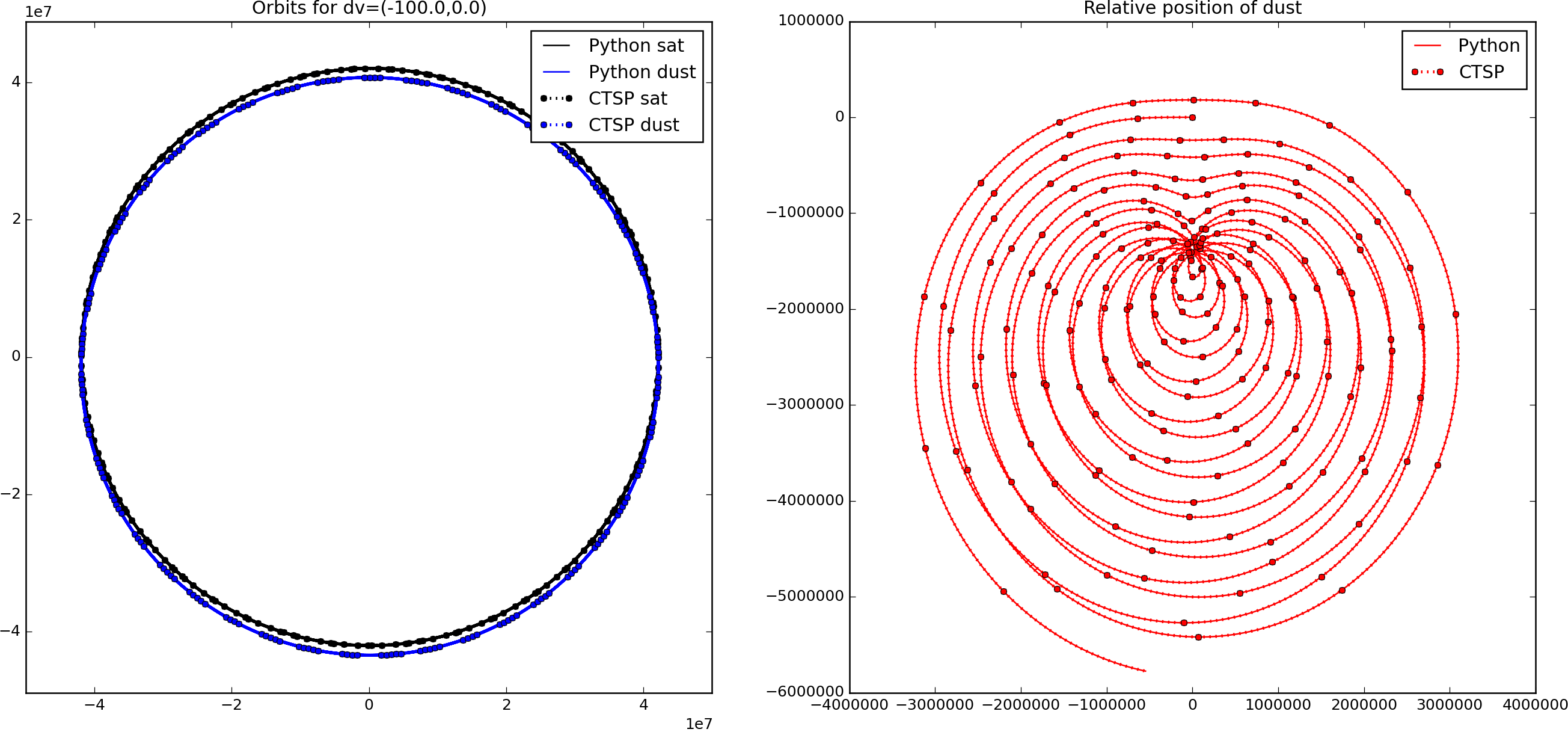
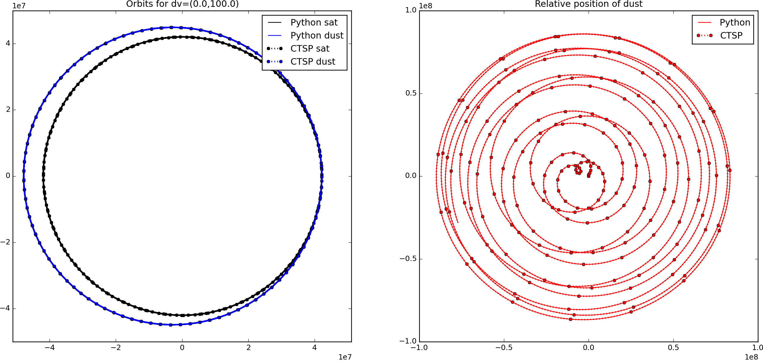
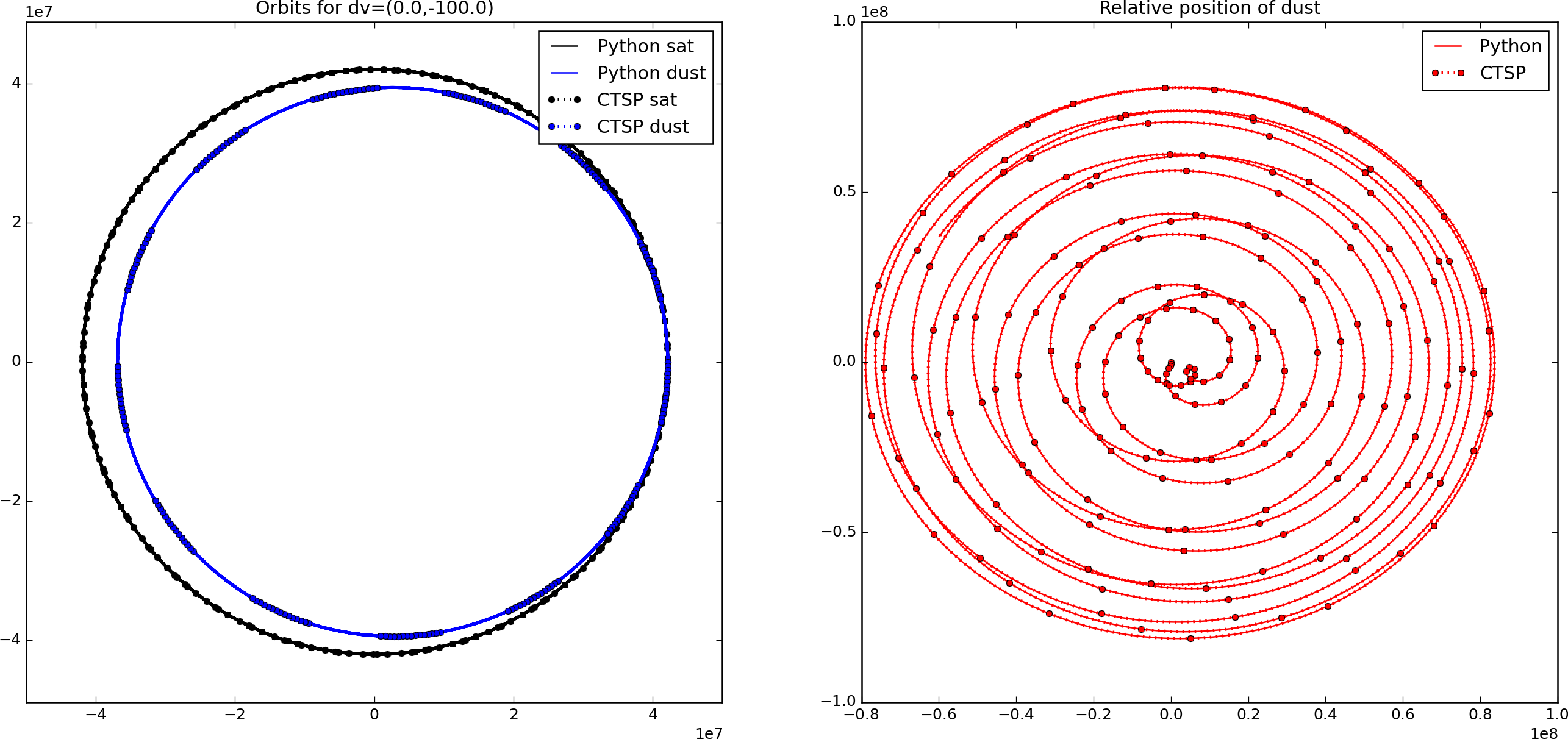
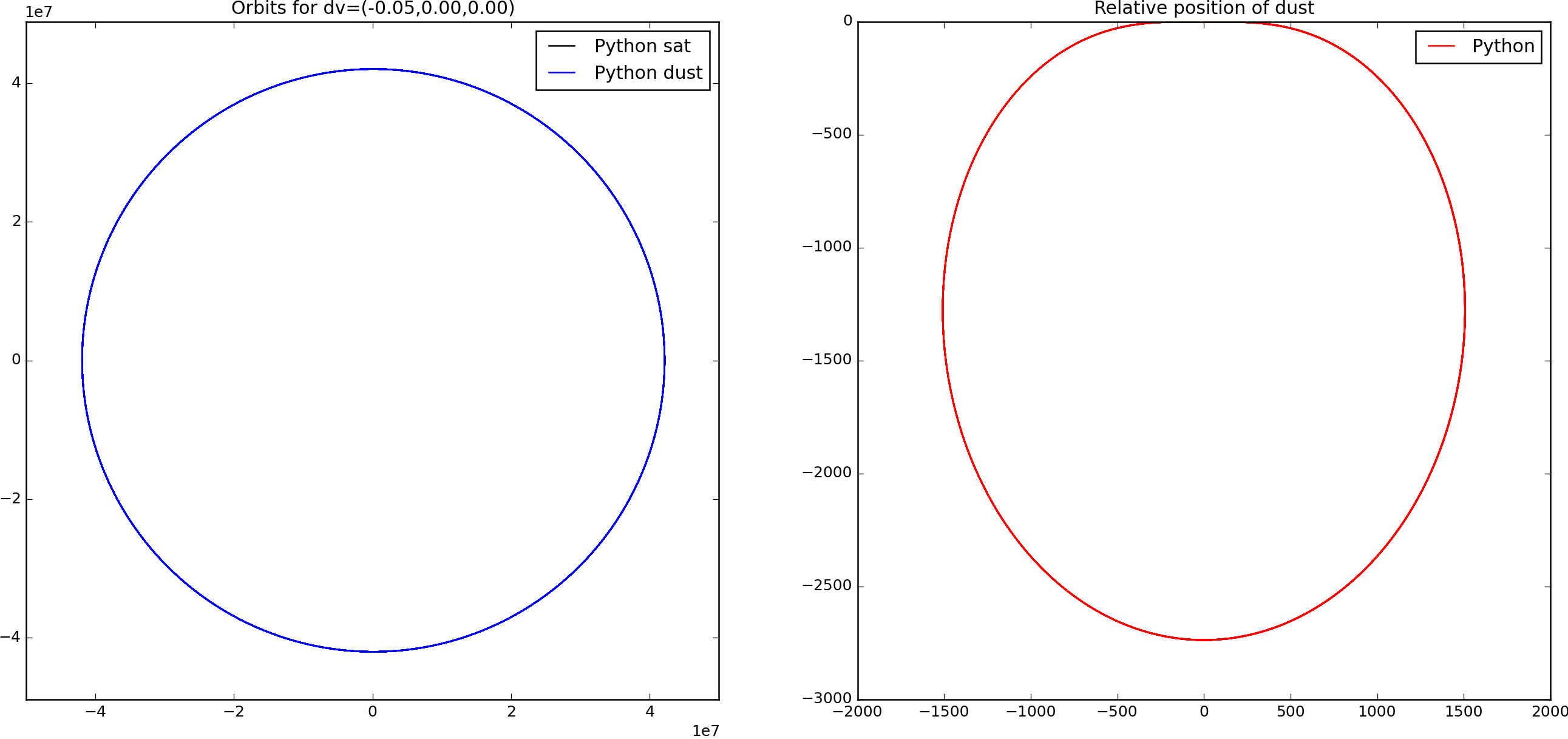
As you can see, the orbit of the dust relative to the satellite can take on some quite funky shapes! However, we don’t really see collisions, but this is due to the large injection velocity. Now, I don’t know at what velocity the particulates leave, but it’s probably closer to centimeters per second, instead of the 100 m/s considered above. When we use 5 cm/s delta velocity, we get the plot as shown below in Figure 3. Now the relative position routinely crosses through the (0,0) point, indicating the particle impacting the satellite.

Solar Pressure

In reality, the relative orbit will not have the shape as shown above due to various perturbations, such as non-uniformities in the gravitational field. I neglected this one. Another effect is drag due to solar pressure. The scalar magnitude at 1 AU is obtained from the following equation
$$P_S=a \frac{W}{c} \cos^2⁡\alpha$$

Here, \(W\) is the solar constant valued at 1361 W/m² and \(c\) is the speed of light. The factor \(a\) has value of 1 for perfectly absorbing surfaces and 2 for reflecting surfaces. A colleague suggested to use 1.4 for diffusely reflecting surface so that’s what I used. The angle \(\alpha\) is the angle between the surface normal and the light incidence angle. In the code, I assumed that the flake, approximated as a flat plate, is randomly tumbling. I hence used an average value over \([-\pi/2:\pi/2]\) range (don’t quote me on this as not sure if this approximation is correct). This can be computed from
$$\overline{\cos^2\alpha}=\frac{1}{\frac{\pi}{2}-\frac{-\pi}{2}}\int_{-\pi/2}^{\pi/2}\cos^2\alpha \text{d}\alpha$$
The “cosine squared” integral is computed using the half angle identity,
$$\begin{align}
\overline{\cos^2\alpha} &= \frac{1}{\pi}\int_{-\pi/2}^{\pi/2}\left(\sqrt{\frac{1+\cos 2\alpha}{2}}\right)^2\alpha \text{d}\alpha\\
&=\frac{1}{2\pi}\int_{-\pi/2}^{\pi/2}1+\cos 2\alpha \text{d}\alpha\\
&=\frac{1}{2\pi}\left[\alpha+\frac{1}{2}\sin 2\alpha \right]_{-\pi/2}^{\pi/2}\\
&=\frac{1}{2}
\end{align}
$$

What’s interesting about solar pressure is that for half of the orbit, it pushes on the particle, while for the half, it pushes against it. This also means we need to know the position of the sun relative to the particle. I used a function from Cowel’s Method for Earth Satellites code by David Eagle to compute the position of the sun in the ECI coordinates. We can then compute the solar radiation pressure force acting on the particle as
$$\vec{F}_S = P_SA \frac{\vec{x}_{p}-\vec{x}_{S}}{|\vec{x}_{p}-\vec{x}_{S}|}$$
where the last term is simply the unit vector denoting the direction from the sun to the particle. Note that in case of the gravitational force, we didn’t actually need the mass of the particle, since that term dropped out when computing \(d\vec{v}/dt\equiv\vec{F}/m\). But we need it to compute the acceleration due to solar pressure. In the code below, I assumed that the dust flake is a brick 1mm x 2mm x 0.5mm with density of 2000 kg/m³. These was just an assumption, so again, don’t quote me on this.

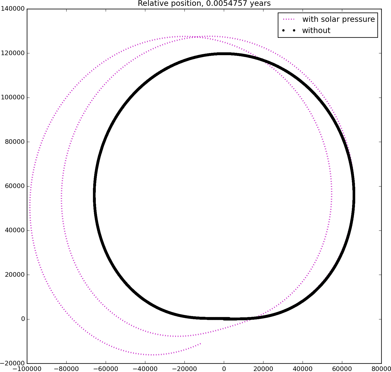
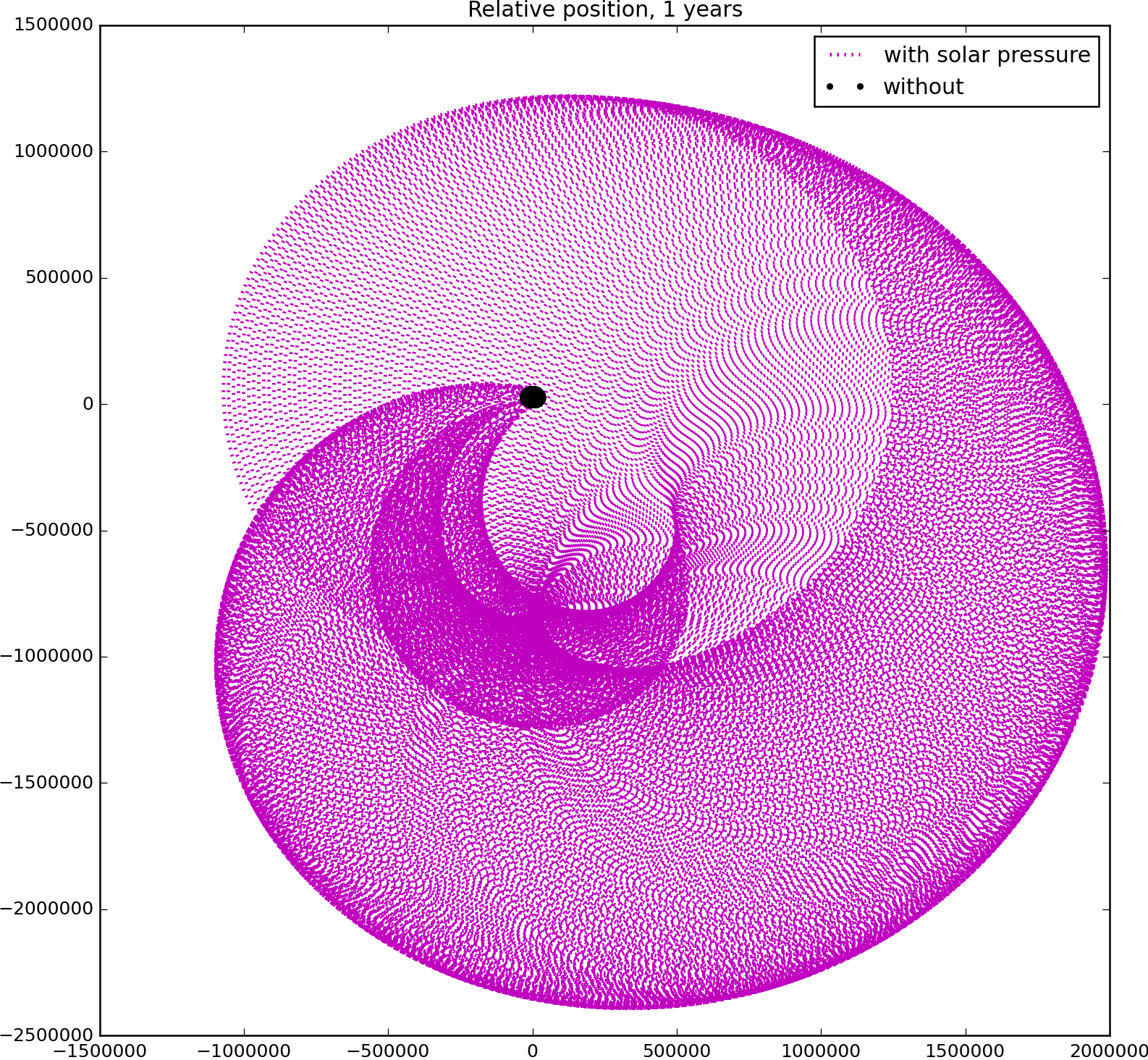
In order to keep this post shorter, I skipped including the text of the second code here, but can find it here: sun.py. When you run this code, you will get a plot like shown in Figure 4. The first figure is result after 2 days, while the second one is after a year. The black line is the unperturbed relative position, while the magenta line corresponds to the result with solar drag. As you can see, they are quite different!

And that’s it. Again, feel free to comment especially if you find some bugs in the code.

Source Code

The source code for the two Python codes is here:
newton.py
sun.py