Vorticity – Stream Function Formulation for Axisymmetric Flow

Few weeks ago, a Reddit user xieta posted really neat results of flow past a cylinder to /r/CFD. These results were computed using the vorticity – stream function method. My background in CFD is quite limited, and to be honest, this was the first time I’ve heard of this method. Turns out it’s a rather popular method for 2D incompressible flows [1].
In 2014, I tried to write my first CFD solver to model purge effectiveness in a cylindrical cavity. Preliminary results from that effort were presented at the SPIE Optics & Photonics conference. That simulation was done using the projection method, and for whatever reason, I just could not get the outflow boundary to behave correctly. This Reddit post had me research the vorticity method as a possible alternative. I found many articles and example codes online, unfortunately, they all seem to be developed for the Cartesian (x-y) coordinates. I was interested in modeling axisymmetric flow, and thus needed formulation in the cylindrical (r-z) system. This article outlines the method I ended up with. Keep in mind that I am in no way a CFD expert. There may be mistakes, and there are likely better ways to treat external boundaries. I am partly posting this article to generate feedback and garner community review, so please leave a comment if something is not right.
Formulation
Velocity Components
 To keep the number of equations to minimum, details of the formulation were moved to a separate pdf. But in brief, for two-dimensional incompressible flows it is possible to express velocity components as derivatives of a scalar “stream” function \(\psi\) such the continuity equation is automatically satisfied. Salih [2] does great job deriving the formulation for a Cartesian flow in which \(u=\partial_y\psi\) and \(v=-\partial_x\psi\). For an axisymmetric flow, we instead use the Stokes stream function,
$$u_z=u=\frac{1}{r}\frac{\partial \psi}{\partial r}\\
u_r=v=-\frac{1}{r}\frac{\partial \psi}{\partial z}$$
Vorticity
Vorticity is defined as \(\omega=\nabla \times \vec{v}\). For axisymmetric flow any \(\partial_\theta=0\) and \(u_\theta\), if present, is independent of the other velocity components. Then,
$$\omega=\omega_\theta=\frac{\partial v}{\partial z} – \frac{\partial u}{\partial r}$$
Stream Function Governing Equation
The definition of velocity components in terms of the stream function can then be substituted into the vorticity equation to obtain
$$ \frac{\partial^2\psi}{\partial z^2} + \frac{\partial^2\psi}{\partial r^2} – \frac{1}{r}\frac{\partial \psi}{\partial r} = -\omega r$$
Note that although this looks like the Poisson’s equation, the sign on the last term on the left hand side is different.
Vorticity Transport Equation
What ties this method to the Navier Stokes equations is the vorticity transport equation. This equation is derived by taking curl of the momentum equation as demonstrated in [2]. For axisymmetric flow it is given by
$$\frac{\partial \omega}{\partial t} + u\frac{\partial w}{\partial z} + v\frac{\partial w}{\partial r} =
\nu\left[
\frac{\partial^2\omega}{\partial z^2} + \frac{\partial^2\omega}{\partial r^2} + \frac{1}{r}\frac{\partial \omega}{\partial r}
\right]$$
Finite Difference Form
The stream function and vorticity equations can be solved using the finite difference method. The stream function equation is discretized using the standard central difference, and can be solved using an iterative elliptic solver, such as Jacobi or Gauss-Seidel. The vorticity equation is a PDE that is marched forward in time. The obvious method is using forward time integration and central space differencing (FTCS). The vorticity transport equation is basically advection-diffusion equation. It can be shown (see [1] or other CFD texts) that the FTCS method is unconditionally unstable for advection equation (inviscid flow). Adding diffusion allows the use of FTCS, but still a restrictive condition on time step remains. I ended up using the 4th order Runge Kutta (RK4) method here. The transport equation is rewritten as \(\partial_t\omega=R(\omega)\) and then three intermediate values of \(\omega\) are computed. Take a look at the pdf for detail.
Boundary Conditions
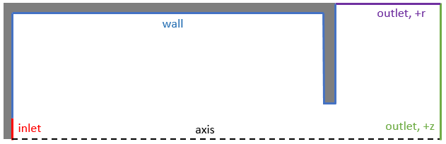
To demonstrate the method, let’s apply it to a flow in cylindrical cavity. The cavity, shown in Figure 1 below, contains inlet on one side. The other side is open to the ambient environment. This setup may look like a simplified version of the SPIE purge problem since that was the intention! We can see that we have five types of boundary conditions to consider. Here I describe them only at top level, again take a look at the pdf for details.
- Inlet: here we assume that flow is parallel with the z axis, giving us \(\partial_z\psi=0\)
- Axis of revolution: there can be now flow across the axis and also \(\partial_r\)=0 so we set \(\psi=0\)
- Solid walls: no slip condition gives us \(\psi=\psi_{wall}\) Dirichlet boundary on walls, with value set from prescribed inlet flow, since \(Q=2\pi\psi\)
- Open boundary on zmax: Here \(\psi\) is set from the definition of velocity and \(\partial_z\omega=0\) is used on vorticity
- Open boundary on rmax: I am not sure what is the appropriate condition here but setting \(u=0\) and \(\partial_r\omega=0\) gives reasonable results
Demo Code in Python
I did most of the initial development in Python. The source code is linked at the bottom of the article. Let’s take a look at the main algorithm. As you surely already noticed, the actual program has additional code here for setting simulation parameters and doing screen output.
#generate geometry
node_type = makeGeometry()

#set streamfunction boundary conditions
psi = initPsi()

#set initial values to zeros
w = np.zeros_like(psi)
u = np.zeros_like(psi)
v = np.zeros_like(psi)

#iterate
print ("Starting main loop")
for it in range (1001):
    #solve psi
    psi = computePsi(w,psi,u,v)

    #update u and v
    u,v = computeVel(psi)

    #advance w
    w = advanceRK4(w,psi,u,v)

    if (it%100==0):
        flux,u_ave = make_plot(it)

print ("Done!")
The first function makeGeometry flags node types as wall, inlet and so on. Then based on these, stream function boundary conditions are set in initPsi. I am setting initial vorticity to zero since the simulation begins with zero flow. The simulation then dives into the main loop. computePsi solves the “Poisson-like” stream function equation using the Jacobi method. Velocity components are then computed in the entire domain by differencing psi. Vorticity transport equation is then marched forward using the RK4 scheme. Finally every 100 iterations, the screen output is updated (this only works if you run the code in Python console).
Here is the RK4 vorticity marcher:
#advances vorticity equation using RK4
def advanceRK4(w,psi,u,v):
    applyVorticityBoundaries(w,psi,u,v)

    #compute the four terms of RK4
    Rk = R(w)
    w1 = w + 0.5*dt*Rk

    R1 = R(w1)
    w2 = w + 0.5*dt*R1

    R2 = R(w2)
    w3 = w + dt*R2

    R3 = R(w3)
    w_new = w + (dt/6.0)*(Rk + 2*R1 + 2*R2 +R3)

    #return new value
    return w_new
First, vorticity is set along all boundaries by calling applyVorticityBoundaries. The R function is used to evaluate \(R=\nu\nabla^2\omega – \vec{v}\cdot\nabla\omega\):
#computes RHS for vorticity equation
def R(w):
    dz2 = dz*dz
    dr2 = dr*dr
    #make copy so we use consistent data
    r = np.zeros_like(w)
    for i in range(1,ni-1):
        for j in range(1,nj-1):
            if (node_type[i,j]>0): continue

            #viscous term, d^2w/dz^2+d^2w/dr^2+(1/r)dw/dr
            A = nu*(
                (w[i-1][j]-2*w[i][j]+w[i+1][j])/dz2 +
                (w[i][j-1]-2*w[i][j]+w[i][j+1])/dr2 +
                (w[i][j+1]-w[i][j-1])/(2*dr*pos_r[j]))

            #convective term u*dw/dz
            B = u[i][j]*(w[i+1][j]-w[i-1][j])/(2*dz)

            #convective term v*dw/dr
            C = v[i][j]*(w[i][j+1]-w[i][j-1])/(2*dr)


            r[i][j] = A - B - C
    return r
Take a look at the source code for the other functions.
Results from Python
Below you will find results from the example Python code after 200 and 1000 time steps. The top plot is the stream function. The bottom half plots flow speed and velocity vectors.


Results from Java purge code
While Python is great for prototyping, I find it too slow for actual simulations with large number of nodes. As such this vorticity – streamfunction method was implemented in the Java purge code. You can see the results below. The flow inside the cavity looks similar (identical?) to the one obtained previously with the projection method but now the external flow also looks right. Success!
Empty Tube
The two videos below show results for an empty tube. They both show the same result, but top plot is on a log scale from 0.002 to 0.16 m/s, while the second one is on linear scale with minimum speed 0.02 m/s.
Tube with Cup and Baffle
Here is the result with the cup and baffle included. Speed is shown on log scale.
Source Code
You can download the source code here: vorticity-rz.py
References
[2] Tannehill, J., Anderson, D., Pletcher, R., Computational Fluid Mechanics and Heat Transfer, Taylor & Francis, 2nd ed., 1997
[2] Salih, A., Streamfunction-Vorticity Formulation, Department of Aerospace Engineering Indian Institute of Space Science
and Technology, March 2013
And that’s it. Again, please leave a comment below. I am very much looking for critiques and review of the boundary conditions. I plan on submitting results from the purge code to a journal soon so this way I hope to catch issues with the CFD solver before the reviewers.
Hi sir
Its a great work u posted here.
It is much useful for my project works
But only one thing is lacking.
The pressure poisson equation in axisym form.
It wil be of much valuable if u post that equation too.
Thankyou again for this post
Regards
Ramkumar
Hi,
the vorticity equation is written with a mistake.
Regards, Vladimir