Starfish DSMC Tutorial: Supersonic Jet and Argon Diffusion

Introduction
This tutorial article will show you how to setup DSMC simulations in Starfish. As you already know, Direct Simulation Monte Carlo is a kinetic method for simulating gas flows. This method collides two actual particles conserving momentum and energy, which is not the case with the alternate MCC approach. DSMC is described in much detail in G.A. Bird’s original text [1], the updated version [2], and his website.
Until recently, DSMC was available only in the full version of Starfish. However, as of version 0.16, it is now available to all! Big reason for not including it earlier was that I did not have a good validation case ready. So when a former student from the plasma simulation courses asked for assistance with a Matlab DSMC code, I saw an opportunity. He was interested in reproducing results from a paper by Jugroot [3] in which the authors used CFD to simulate expansion of ambient pressure nitrogen gas to a low pressure tank in a mass spectrometer. As the authors noted,
The Knudsen number … can become relatively large in the high-Mach-number and low-pressure regions of the interface flows downstream of the orifice. This would imply that non-continuum and thermal non-equilibrium effects may be significant in these regions and that a continuum fluid dynamic model may not be strictly valid. Nevertheless, as a first step towards improving the understanding of interface flows in mass spectrometers, it is felt that a near-equilibrium continuum model is sufficiently accurate. It should be noted that non-continuum effects in high-speed expanding flows will primarily influence the thermal structure of the gas, but dynamic features such as velocity and density distributions and overall flow structure are not strongly affected.
In this tutorial we will see how to set up this problem. We will also reproduce a self-diffusion of Argon example from [1].
Starfish DSMC Formulation
I first need to mention some important points about the DSMC implementation in Starfish. The algorithm is heavily based on Bird’s original DSMC0.FOR code. However, there are three notable differences. First, the code uses only the prescribed mesh cells to group particles. Modern DSMC codes instead use automatically generated “collision cells” with cell size scaling automatically with local density. This is a very important feature that I will try adding in a future version. The issue is that if mesh cells are too small, there may be cells with fewer than two particles at any given time, and thus collisions won’t be possible. On the other hand, if cells are too large, particles may collide that are physically too far apart for collision to take place. Second, the code does not model vibrational or rotational energies. Thus molecular gas is treated as monoatomic gas, just with larger atoms. Again, this is something to be added in the future. And thirdly, instead of using Bird’s No Time Counter (NTC) scheme, the number of collision pairs is selected based on a paper of Boyd [4],
$$ N_c = \frac{(N_a/\Delta V)N_b\Delta t (\sigma g)_{max}}{P_{a,b} + (W_b/W_a)P_{b,a}} $$
where \(P_{a,b}=\max(W_b/W_a,1)\) and \(P_{b,a}=\max(W_a/W_b,1)\). This formulation allows the code to model collisions between species having different macroparticle weights (the number of real particles represented by each simulation particle). Bird’s NTC scheme requires both colliding species to have the same weight, which can lead to difficulties when modeling real engineering problems. There are two approaches for dealing with variable weights. One is to split the more massive macroparticle into two particles, with one having the same weight as the collision target. Momentum can then be conserved in each collision. The problem with this conservative method is that it can lead to a growth in the number of simulation particles unless some merging algorithm is applied. The alternative is to alter velocities of the more massive particle only at a rate corresponding to the ratio of particle weights,
/*variable weight*/
double Pab = part2.spwt/part1.spwt;
double Pba = part1.spwt/part2.spwt;

if (Starfish.rnd()<Pab)
    for (int i=0;i<3;i++)
        part1.vel[i] = vc_cm[i]+rm2*vr_cp[i];

if (Starfish.rnd()<Pba)
    for (int i=0;i<3;i++)
        part2.vel[i] = vc_cm[i]-rm1*vr_cp[i];
In other words, if particle “A” simulates 10x as many real molecules as particle “B”, we alter post-collision velocities of “A” only 1 every 10 times. This method is nonconservative since for non equal weights, momentum will be conserved only on average at steady state. Using this method requires changes to the number of collision pairs to be selected, which is what Boyd’s equation accomplishes. For \(W_a=W_b\), the scheme reduces back to Bird’s original NTC algorithm. This is the method currently implemented in Starfish.
Example 1: Supersonic Jet Expansion
The first example attempts to replicate setup from [3]. The authors were interested in simulating nitrogen gas expanding from a 750 Torr (basically atmospheric) environment to a 0.5 Torr tank through a 0.75mm diameter orifice. This is an axisymmetric problem. With the orifice exit plane centered at (0,0), their simulation domain extended to 25 mm in the axial direction and 11 mm in the radial direction. They didn’t specify what kind of mesh was used but listed the typical number of cells as 50,000. I set up the problem with a uniform Cartesian mesh with 1e-4 node spacing and 27,500 cells in the low pressure region. Since I wanted to keep the orifice boundary aligned with a mesh edge, the orifice diameter was increased slightly to 0.8mm.
The setup for this problem is visualized in Figure 1 above. We will use ambient sources to maintain constant pressure along the red and orange boundaries. This source simply creates particles while pressure in the neighboring cell is below some user given threshold. Particles are sampled as thermal gas but can be given optional drift velocity. Besides maintaining pressure, the source can also maintain density. These two properties are related by the ideal gas law, \(P=nkT\). The black boundary is a solid wall diffusely reflecting incident molecules. Temperature of this wall will be set to the same temperature as the injected gas. Figure 1 shows results after 200 time steps. As you can see, we start with an initially empty domain. I experimented with prefilling the low density region with the 0.5 Torr gas but found it to make no difference.
Input Files
We will now go through the input files needed by the simulation. You will find them in the dat/dsmc/jet directory.
We start with the main starfish.xml file. As you can see, it’s quite short. We tell the simulation to run for 70,000 time steps, with steady state forced at time step 20,000. This controls when averaging begins. The automatic steady state checking code is not robust, and I wanted to make sure we are truly at steady state when we start collecting data. I also included optional restart code. One other thing you may note is a lack of code specifying averaging. As of v0.16, velocities, density, and temperature are automatically averaged for kinetic species.
<simulation>
<note>DSMC gas expansion</note>
<log level="Log" />

<!-- load input files -->
<load>domain.xml</load>
<load>materials.xml</load>
<load>boundaries.xml</load>
<load>interactions.xml</load>
<load>sources.xml</load>

<!-- set time parameters -->
<time>
<num_it>70000</num_it>
<dt>1e-8</dt>
<steady_state>20000</steady_state>
</time>

<!--
<restart>
<it_save>5000</it_save>
<save>true</save>
<load>false</load>
<nt_add>500</nt_add>
</restart>
-->

<!-- run simulation -->
<starfish/>

<!-- save results -->
<output type="2D" file_name="field.vts" format="vtk">
<variables>nodevol, p, nd-ave.n2, t.n2, t1.n2, t2.n2, t3.n2, u-ave.n2, v-ave.n2, w-ave.n2, nu, mpc.n2, dsmc-count</variables>
</output>

<output type="boundaries" file_name="boundaries.vtp" format="vtk">
<variables>flux.n2, flux_normal.n2</variables>
</output>

</simulation>
The variables that we are outputting include node volume, total pressure, average number density of nitrogen, total temperature, temperature components for the three spatial directions, average velocity components, collision rate, average number of macroparticles per cell, and average number of collisions per cell. All this data is saved as point data. In the future, I will make the output algorithm more user friendly by having it save velocity components directly as vectors.
The domain.xml file specifies the uniform mesh used for particle push, collisions, and sampling:
<domain type="zr">
<mesh type="uniform" name="mesh">
<origin>-5e-4,0</origin>
<spacing>1.0e-4, 1.0e-4</spacing>
<nodes>256, 111</nodes>
<mesh-bc wall="bottom" type="symmetry"/>
</mesh>
</domain>
It is not necessary to specify symmetry on the \(r=0\) edge for an axisymmetric code (domain type="zr") but I left it here in case you want the run the code in the xy mode (domain type="xy")
The materials.xml file lists known materials used for specifying boundaries and gas particles,
<materials>

<material name="N2" type="kinetic">
<molwt>28</molwt>
<charge>0</charge>
<spwt>1e11</spwt>
<ref_temp>275</ref_temp>;
<visc_temp_index>0.74</visc_temp_index>
<vss_alpha>1.00</vss_alpha> <!--1.36-->
<diam>4.17e-10</diam>
</material>

<material name="SS" type="solid">
<molwt>52.3</molwt>
<density>8000</density>
</material>

</materials>
The file lists two materials: nitrogen molecules and stainless steel for surfaces. One important thing to note here is that for a kinetic material (flying gas particles) we also specify various DSMC parameters. These values for nitrogen come from Tables A1, A2 and A3 in Appendix A of Bird’s 2003 book. The vss_alpha can be used to turn on the Variable Soft Sphere (VSS) collision model. Value of 1 results in the faster Variable Hard Sphere (VHS) being used. I ran few cases and did not observe any significant differences between the two and hence we’ll be using VHS in this example. You can speed up the code by using a higher specific weight with the risk of adding numerical error due to not having enough particles per cell.
The boundaries.xml file specifies surface boundaries in an SVG format. You could generate the segments for complex geometries using “path to SVG” in GIMP or Inkscape, but for a simple geometry, you can just make the file by hand,
<boundaries>

<boundary name="wall" type="solid">
<material>SS</material>
<path>M 0, 11e-3 L 0,8e-4 -1e-3,8e-4</path>
<temp>288</temp>
</boundary>

<boundary name="inlet" type="solid">
<material>SS</material>
<path>M wall:last L -1e-3,0</path>
<temp>288</temp>
</boundary>

<boundary name="ambient" type="virtual">
<path>M 25e-3,0 L 25e-3,11e-3 0,11e-3</path>
</boundary>

</boundaries>
The “ambient” boundary is marked as virtual. This allows this boundary to be used when specifying particle sources but is subsequently invisible to particles during the push. Although “inlet” is marked as solid, it doesn’t seem to make a difference. A virtual inlet means that a particle moving back to the tank is removed, and subsequently new particle is generated by the ambient source. However, since both use the same algorithm to sample a half Maxwellian, the result is the same.
Particles sources are listed in the sources.xml file,
<sources>

<!--high pressure tank-->
<boundary_source name="inlet_750Torr" type="ambient">
<enforce>pressure</enforce>
<material>N2</material>
<boundary>inlet</boundary>
<drift_velocity>0,0,0</drift_velocity>
<temperature>288</temperature>
<total_pressure>1.0e5</total_pressure>
</boundary_source>

<!--ambient environment-->
<boundary_source name="amb_0.5Torr" type="ambient">
<enforce>pressure</enforce>
<material>N2</material>
<boundary>ambient</boundary>
<drift_velocity>0,0,0</drift_velocity>
<temperature>288.0</temperature>
<total_pressure>66.66</total_pressure>
</boundary_source>

</sources>
As you can see, we are specifying two sources of type ambient. This source attempts to maintain constant density, pressure, or partial pressure (as given by the enforce parameter) in cells along the given boundary. Particles are sampled from a half-Maxwellian at the given temperature (288K). The first source generates particles for the 750 Torr reservoir, while the second source generates particles to fill the low pressure tank. Pressures are given in Pascal, hence values in Torr need to be multiplied by 133.322.
Finally, we have interactions.xml file, which specifies particle-surface and particle-particle interactions,
<material_interactions>
<surface_hit source="N2" target="SS">
<product>N2</product>
<model>diffuse</model>
<prob>1.0</prob>
</surface_hit>

<dsmc model="elastic">
<pair>N2,N2</pair>
<sigma>Bird463</sigma>
</dsmc>

</material_interactions>
This file tells the simulation that a nitrogen molecule hitting a stainless steel surface should reflect diffusely. Collisions between nitrogen molecules are handled with DSMC, with the collision cross-section given by Equation 4.63 in [1],
$$ \sigma = \pi d^2 \\d = d_{ref} \left(\frac{\left[2kT_{ref}/(m_r c_r^2)\right]^{\omega-1/2}}{\Gamma(5/2-\omega)} \right)^{1/2}$$
Results
To run the code, navigate to the directory with the input files and execute
java -jar starfish-LE.jar
from the command line (this assumes starfish-LE.jar is in that folder). I actually ran these simulations on Amazon Web Services, since these runs will take maybe 12 hours to finish. On AWS, you may want to run the code in background with nohup so the job doesn’t terminate when you log out,
nohup java -jar starfish-LE.jar &
Once the simulation finishes, you will have a file called field.vts which you can visualize using Paraview. For now, all results are saved as node-centered data. In order to visualize streamlines, we need to use Paraview’s calculator filter to generate vectors. This is done with the following equation: u-ave.n2*iHat+v-ave.n2*jHat and the result is saved in variable vel. We also need to compute Mach number, \(M=|v|/\sqrt{\gamma kT/m}\). Add another calculator to the output from the above calculator and use mag(vel)/sqrt(1.4*1.3806e-23*t.n2/(28*1.661e-27)) to compute result
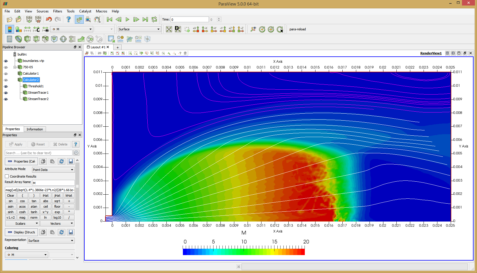
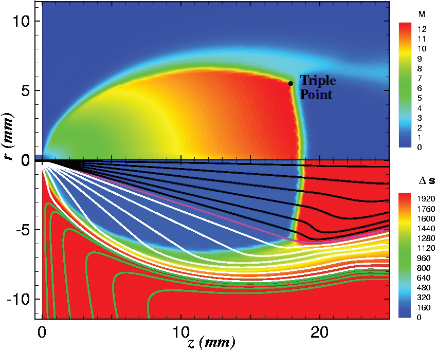
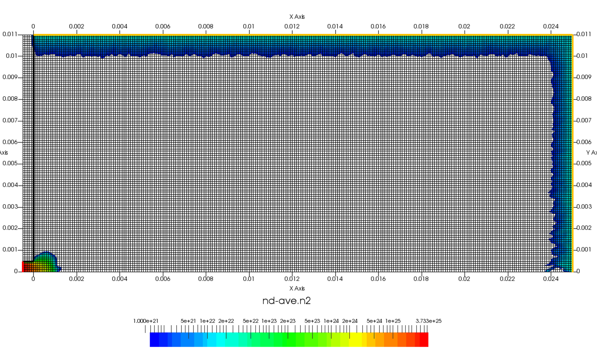
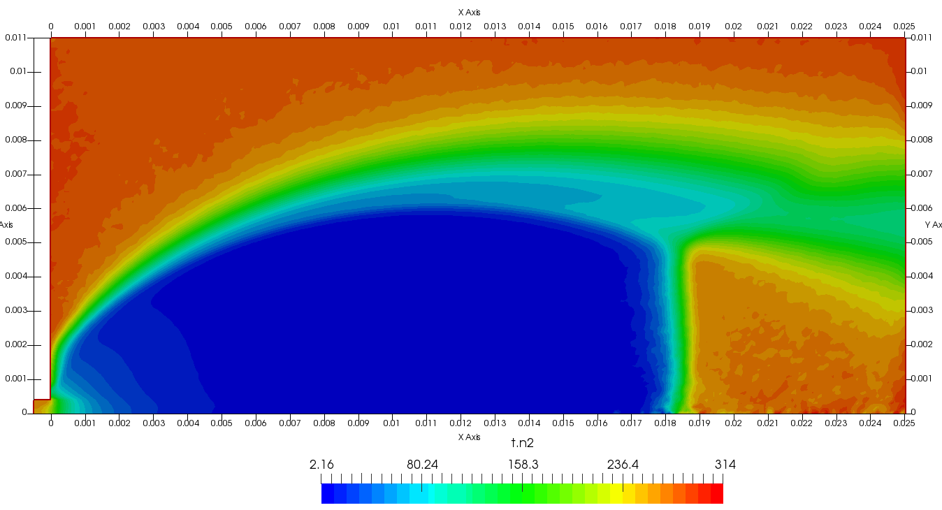
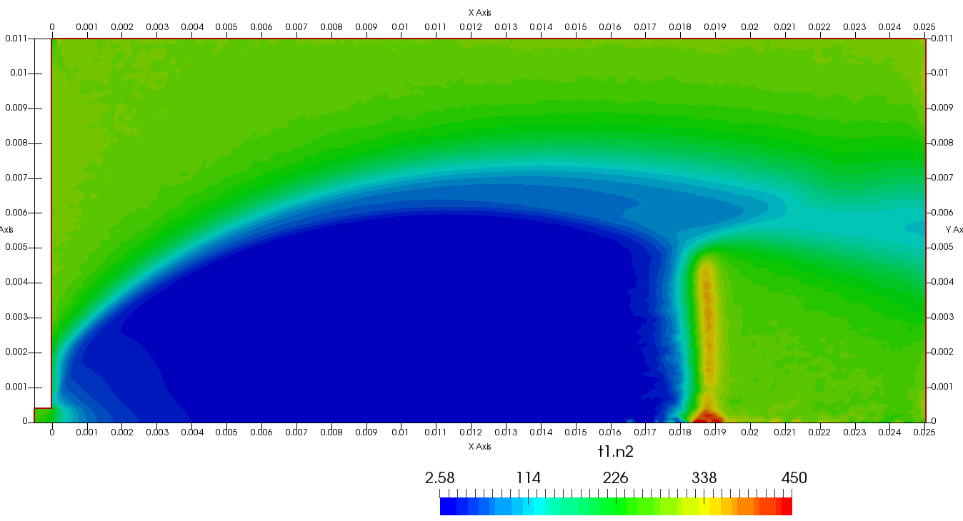
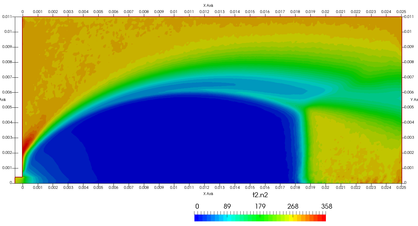
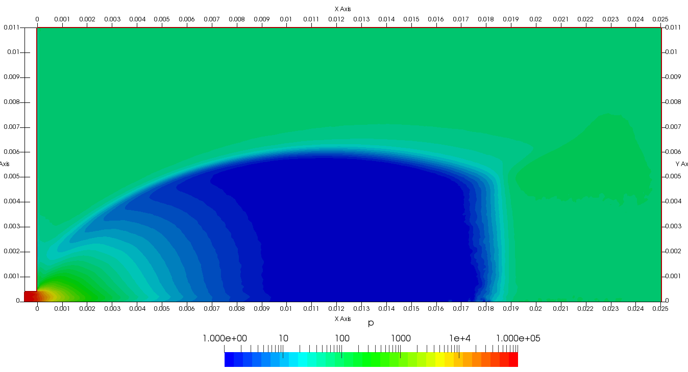
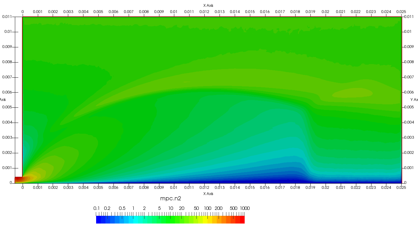
Figure 4 plots number density and Figure 5 plots total temperature computed by sampling particle velocities. Temperatures in the axial and radial direction are shown in Figure 6. We can note the as expected, the supersonic jet starts cooling as it expands. From ideal gas law, we can also compute pressure, which is shown in Figure 7. Pressure decays to sub 1 Torr in the jet, but then rapidly returns to the abmient value across the shock.
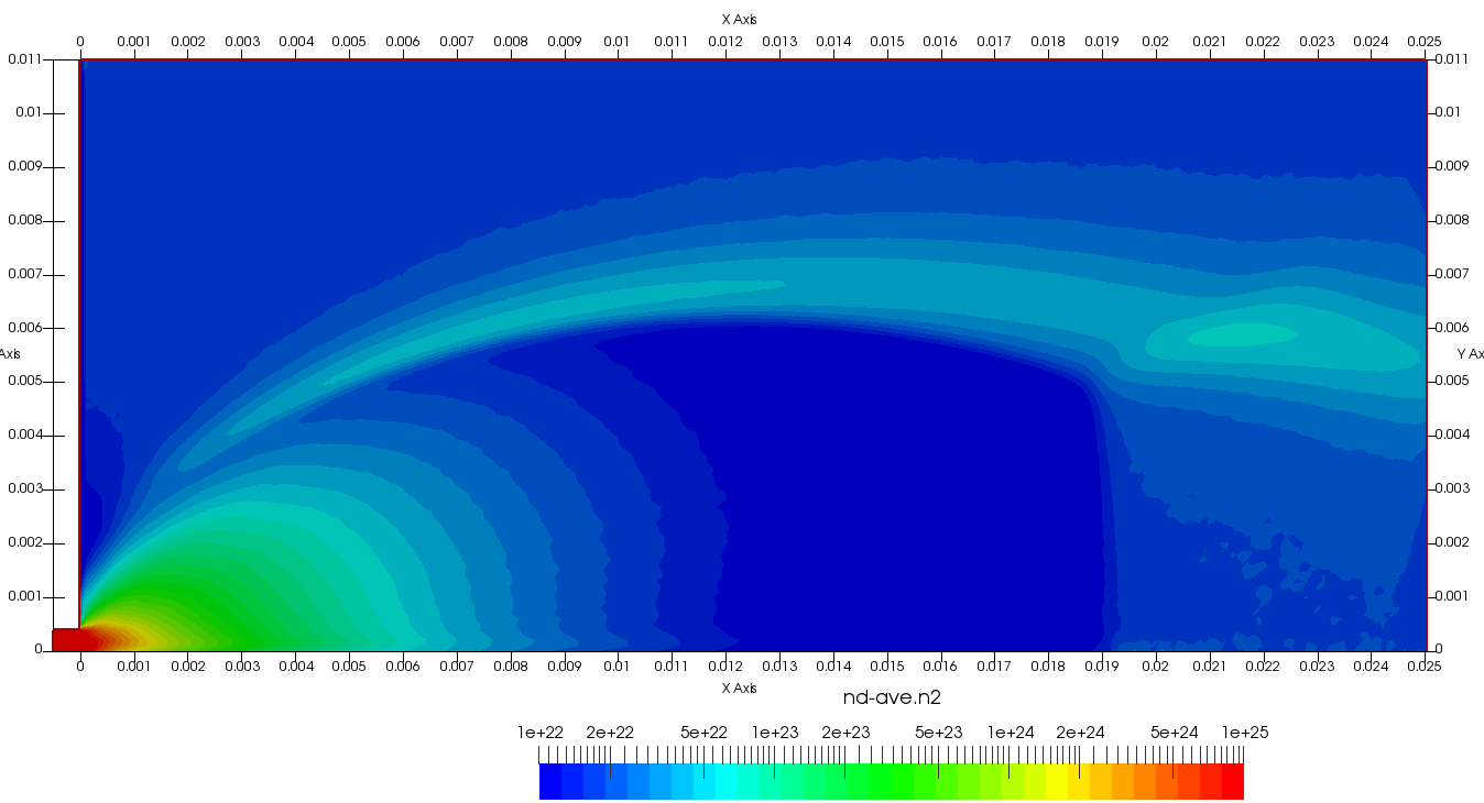
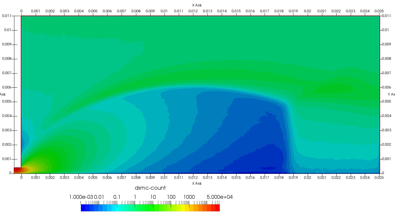
Upon a closer inspection of results, specifically number density or pressure, you may notice some non-physical ripples near the centerline. This is an unfortunate side-effect of the kinetic simulation using uniform mesh and fixed specific weight in an axi-symmetric problem. Cell volumes decrease as we get closer to the axis of rotation, resulting in the simulation not having sufficient number of particles in those cells. We can confirm this from the macroparticle count plotted in Figure 8. We can see that a large fraction of the jet has on average fewer than two particles per cell. Due to the use of uniform mesh for collision grouping, we end up with many cells where collisions cannot be computed.. For now, the only solution is to run the simulation with more particles (which means longer run time). In the future, I anticipate implementing generation of adaptive collision cells. The actual number of collisions per cell is shown in Figure 9.
Example 2: Self-Diffusion Coefficient of Argon
The second example computes the self-diffusion coefficient of argon per pages 271-273 of [1]. You will find these input files in dat/dsmc/diffusion. We model two argon tanks placed 1 m apart, with gases from each allowed to mix in a cavity joining them. The speed with which molecules from one tank diffuse to the other population can be used to calculate the diffusion coefficient. Bird notes that different isotopes are used in experiments. Numerically, or task is easier. We simply use two different species, ar1 and ar2. Except for their names, the two materials have otherwise identical properties,
<!-- materials file -->
<materials>

<!-- data from Bird's Appendix A-->
<material name="Ar1" type="kinetic">
<molwt>39.94</molwt>
<charge>0</charge>
<spwt>5e11</spwt>
<ref_temp>273</ref_temp>;
<visc_temp_index>0.81</visc_temp_index>
<vss_alpha>1.00</vss_alpha> <!--1.40-->
<diam>4.17e-10</diam>
</material>

<material name="Ar2" type="kinetic">
<molwt>39.94</molwt>
<charge>0</charge>
<spwt>5e11</spwt>
<ref_temp>273</ref_temp>;
<visc_temp_index>0.81</visc_temp_index>
<vss_alpha>1.00</vss_alpha> <!--1.40-->
<diam>4.17e-10</diam>
</material>

<material name="SS" type="solid">
<molwt>52.3</molwt>
<density>8000</density>
</material>

</materials>
Interactions between these two are listed in interactions.xml,
<material_interactions>

<dsmc model="elastic">
<pair>Ar1,Ar2</pair>
<sigma>Bird463</sigma>
<frequency>5</frequency>
</dsmc>

</material_interactions>
Note that we are using frequency tag to compute collisions only every 5 time steps. This was bit of a trade off between using a smaller time step to minimize a sampling issue on domain boundaries, and the code running too slowly due to computing collisions too often.
Our domain.xml file uses symmetry on top and bottom edge to create a 1D domain,
<domain type="xy">
<mesh type="uniform" name="mesh">
<origin>0,0</origin>
<spacing>0.02, 0.02</spacing>
<nodes>51, 11</nodes>  <!-- 41 in short-->
<mesh-bc wall="bottom" type="symmetry"/>
<mesh-bc wall="top" type="symmetry"/>
</mesh>
</domain>
boundaries.xml specifies two vertical edges used to sample particles on left and right domain boundary. Note that left edge goes from top to bottom, while right edge is bottom to top to keep both normals pointing inward.
<boundaries>
<boundary name="left" type="virtual">
<material>SS</material>
<path>M 0, 0.2 L 0 0</path>
<temp>273</temp>
</boundary>

<boundary name="right" type="virtual">
<material>SS</material>
<path>M 1.0, 0 L 1.0 0.2</path>
<temp>273</temp>
</boundary>

</boundaries>
The ambient source is used to sample particles once again. This time we will be enforcing density.
<sources>

<boundary_source name="left" type="ambient">
<enforce>density</enforce>
<material>Ar1</material>
<boundary>left</boundary>
<drift_velocity>0,0,0</drift_velocity>
<temperature>273</temperature>
<density>1.4e20</density>
</boundary_source>

<boundary_source name="right" type="ambient">
<enforce>density</enforce>
<material>Ar2</material>
<boundary>right</boundary>
<drift_velocity>0,0,0</drift_velocity>
<temperature>273</temperature>
<density>1.4e20</density>
</boundary_source>

</sources>
Finally, the main simulation starfish.xml file is listed below,
<simulation>
<note>Self diffusion coefficient of Argon</note>
<log level="Log" />

<!-- load input files -->
<load>domain.xml</load>
<load>materials.xml</load>
<load>boundaries.xml</load>
<load>interactions.xml</load>
<load>sources.xml</load>

<!-- set time parameters -->
<time>
<num_it>50000</num_it>
<dt>2e-6</dt>
<steady_state>5000</steady_state>
</time>

<restart>
<it_save>10000</it_save>
<save>true</save>
<load>false</load>
<nt_add>20000</nt_add>
</restart>

<!-- run simulation -->
<starfish/>

<!-- save results -->
<output type="2D" file_name="field.vts" format="vtk">
<variables>nodevol, p, nd-ave.ar1, t.ar1, u-ave.ar1, nd-ave.ar2, t.ar2, u-ave.ar2, mpc.ar1, mpc.ar2, dsmc-count, nu</variables>
</output>

<output type="boundaries" file_name="boundaries.vtp" format="vtk">
</output>

</simulation>
Results
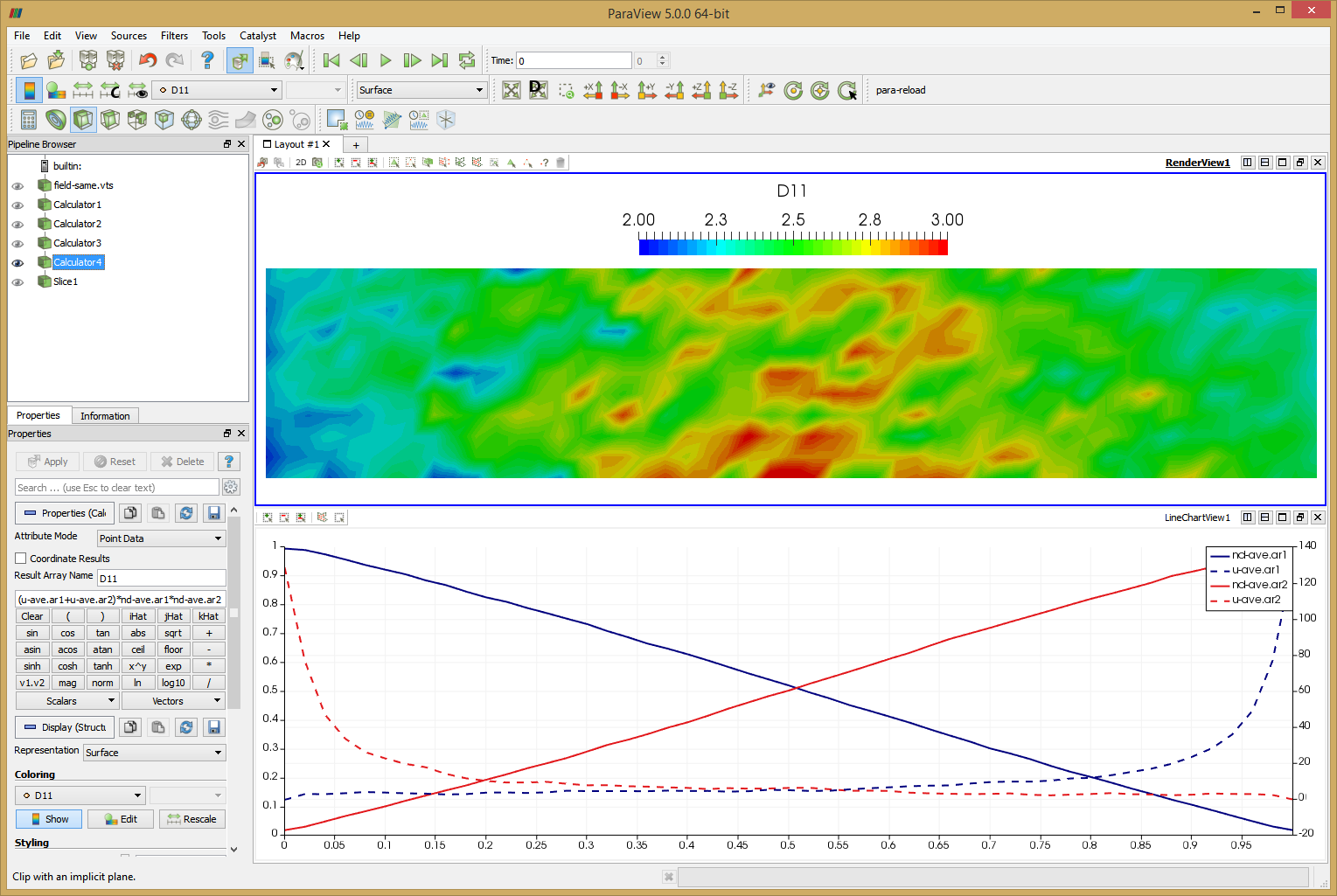
Again, run the code using java -jar starfish-LE.jar. This simulation should take about 2 hours to complete. Feel free to adjust the number of time steps as needed. Again we use Paraview to view the results. I added several calculators to the pipeline. First two were used to normalize the number density by the tank density, nd-ave.ar1/1.4e20 -> nd-ave.ar1. I then flipped the sign of the ar2 velocity since it’s flowing in the negative direction, from right to left, -u-ave.ar2 -> u-ave.ar2. Finally, the diffusion coefficient is computed using the formula given by Bird,
$$D_{11}=-(U_1-U_2)\frac{n_1n_2}{n^2}\frac{\Delta x}{\Delta (n_1/n)}$$
The last term reduces to -1 due to the problem setup. Since the sign of U2 was already reversed and densities are normalized, the formula reduces to (u-ave.ar1+u-ave.ar2)*nd-ave.ar1*nd-ave.ar2 -> D11. You can see this field plotted in the Figure 10 below. Bird computed average value of 2.95. The average I obtained over the entire domain is 2.53. The two results are clearly not identical, but they are quite close. Judging from the noise and non-uniformity in the data, it’s possible this case could benefit from a longer run with more particles. The line plot data shows data along the centerline. This plot can be compared to Figures 12.9 and 12.10 in Bird’s book. Another anomaly that you may notice is that the two density curves don’t cross exactly at 0.5. This is due to statistical error and/or the ambient source. As you run the simulation, you will notice that the particle counts for the two species are not identical. Typically one species may have some 5-10% more particles and after some time, the situation reverses.
Non-equal Macroparticle Weights
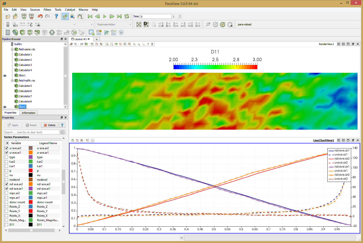
This setup also lets us test the variable specific weight sampling algorithm of Bird. I next doubled the specific weight of ar1 so that there were only half as many ar1 molecules as previously by setting
<material name="Ar1" type="kinetic">
...
<spwt>5e13</spwt>
...
</material>
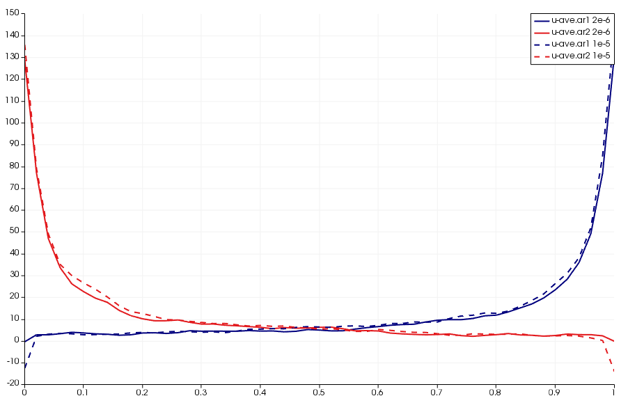
Results from this run are shown below in Figure 11. The line chart has the new results over laid over the old one. The new data is the one with the “crosses”. As you can see, the two results agree with each other.
Sampling
This setup also helped me identify a bug that has yet to be resolved. If you increase the time step 5x to 1e-5 and reduce the dsmc_frequency to 1, you will get results as shown below. The error is the sharp decrease in velocities along boundary nodes. The only difference between these two cases is that particles now take only a single step between “sampling” used to compute macroscopic properties such as density, velocities, and temperature from particle data. Starfish currently discards particles that leave the mesh and thus their properties will not be included in the sample. As such, I suspect that with the larger time step, some of the faster particles are leaving the domain at a higher rate and thus are preferentially not included in the sample. This is yet another bug for me to look into, but perhaps the code needs to sample particles leaving the domain before removing them from the simulation.
References
[1] Bird, G.A., Molecular Gas Dynamics and the Direct Simulation of Gas Flows, Oxford Science Publications, 2003
[2] Bird, G.A, The DSMC Method, CreateSpace, 2013
[3] Jugroot, M., Groth, C., Thomson B., Baranov V., Collings, B., Numerical investigation of interface region flows in mass spectrometers: neutral gas transport”, J. of Phys., D: Applied Physics, vol. 37, pp. 1289–1300, 2004
[4] Boyd, I. D., “Conservative Species Weighting Scheme for the Direct Simulation Monte Carlo Method”, J. Thermophysics and Heat Transfer, Vol. 10, No. 4, 1996
Professor,
when I run the jet case provided by starfish(download from the “CODES”),at last, the screen shows
“it:69999 N2:211364”
Processing
WARNING: Skipping unrecognized variable nu
Processing
Saving restart dat
WARNING: savaRestartData not yet implemented for SS
Done!
I can’t find the output file.why? THANK YOU.
Hi Peter, there should be a “results” folder containing all these files. Is it not there?
Thanks Professor, I didn’t find the “results” folder. Instead, I found some output file in the current folder; It contains the following file:
boundaries.vtp
boundaries.xml
coordinate.txt
domain.xml
domain.xml.bak
field.pvd
field_mesh.vts
interactions.xml
materials.xml
restart.bin
sources.xml
starfish.jar
starfish.log
starfish.xml
starfish_stats.csv;
And I draw some picture using ParaView,it similar to your original version. I guess maybe the way i use to run the code is wrong? I put the starfish.jar into the
“D:\dat\dsmc\jet1fail1103\”, and then i type the command line, “java -jar starfish.jar”, after maybe 6 hours, i got these files. Should I use another way to get the “results” folder you mentioned?
Hi professor I got another question, if i change the pressure on the left boundary(inlet) into 7torr, change the pressure of the right side (the tank) into 0.0001Pa, can i use the mode to caculate this case? I’m not sure whether the mode is suitable to this case. Maybe I suppose to modify more xml files except the sources.xml?
Besides, learning starfish is very happy, thanks for your online courses.
Professor, when I run the case “D:\starfish\dat\IEEEfullpic\central” you provided in starfish, the dos always show the following information, is it correct? thank you!
“WARNING: !! GS failed to converge in 2000 iteration, norm = 0.00104255566899255
44
it: 31671 O+: 596988 e-: 108523
WARNING: !! GS failed to converge in 2000 iteration, norm = 0.00178382109454580
31
it: 31672 O+: 597006 e-: 108499
WARNING: !! GS failed to converge in 2000 iteration, norm = 0.00271099112778573
93”
I think there is a typo in the definition of P_{ab} and P_{ba} (right after 1st equation).