Multigrid Solver

Previously on this blog we saw how to obtain a numerical approximation to the Poisson’s equation \(\nabla^2\phi =b \) using the Finite Difference or Finite Volume method. In 1D, Finite Difference gives us
$$ \frac{\phi_{i-1} -2\phi_i + \phi_{i+1}}{(\Delta x)^2} = b_i$$
We can then solve this linear system using an iterative scheme such as Gauss-Seidel. We simply loop over the nodes over and over, each time computing a new approximation of the node value at iteration \(n\) from
$$ \phi_i^{n+1} = \frac{1}{2}\left( \phi_{i-1}^{n+1} + \phi_{i+1}^{n} – (\Delta x)^2 b_i\right)$$
Motivation
While this method is simple to implement, it is very slow to converge. To see why, let’s consider a system with
$$b = A \sin\left(\frac{k2\pi x}{L}\right)$$
where \(A\) is some magnitude, \(k\) is an integer wave number, and \(L\) is the domain length. In 1D, we have
$$\frac{\partial^2\phi}{\partial x^2} = A \sin\left(\frac{k2\pi x}{L}\right)$$
We can integrate this system analytically subject to boundary conditions,
$$\frac{\partial \phi}{\partial x} = -A \cos\left(\frac{k2\pi x}{L}\right) \left(\frac{L}{k2\pi}\right) +C_1$$
$$\phi = -A \sin\left(\frac{k2\pi x}{L}\right) \left(\frac{L}{k2\pi}\right)^2 +C_1 x + C_2$$
Prescribing the Neumann zero boundary condition \({\partial \phi}/{\partial x}=0\) on \(x=0\) and the Dirichlet \(\phi=0\) on \(x=L\), we obtain
$$C_1 = A\left(\frac{L}{k2\pi}\right)$$
and
$$C_2 = -C_1 L$$
Since we have the analytical solution, we can compute the actual error vector \(\epsilon \equiv (\phi^n – \phi)\) at each iteration. Note that normally you wouldn’t have this option since the solution is not known a priori – otherwise there would be no need to solve the system! In Figure 1 we graph this \(\epsilon\) term over the first 50 iterations (left) or over the entire solution cycle (right) for \(A=10\) and \(k=4\).
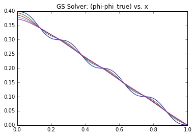
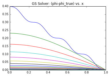
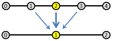
What you can notice right away is that initially there is a high frequency error that dissipates quite quickly. After this, what remains is a low frequency term that takes much longer to reduce. You can think of the high frequency term as the node-to-node variation. The Poisson’s equation specifies the second derivative (the “acceleration”) of \(\phi\). This high frequency term corresponds to how well the local trends are represented – whether the value from node to node “accelerates” correctly. However, just because this local behavior is captured doesn’t mean that the entire solution is right. A Dirichlet boundary is needed to “ground” the system, otherwise we would not have a unique solution. So while the node values may be growing or shrinking correctly node to node, the overall solution may be satisfying a different set of boundary conditions. This implies that the entire solution needs to scale up or down. This is the low frequency term. Because our Finite Difference scheme is based on a three point stencil (in 1D), it takes long time for the boundary information to propagate. In the picture below, you can see that four solver iterations are needed for the highlighted yellow node to even become aware of the boundary.
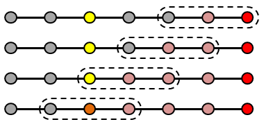
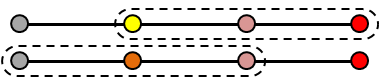
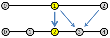
This is the motivation behind multigrid schemes. Since we are after the “global” behavior, it makes sense to advance the solution using a coarser grid. This way, we are effectively stretching the “arms” of the stencil, allowing it to use data farther away. Using a coarse mesh with a doubled mesh spacing ends up halving the number of iterations needed to propagate the boundary value to two.
Error Vector
While it may seem natural to continue by solving the system on the coarser grid, this is actually not the best approach. We don’t care for the actual solution of the original linear system on the coarse grid. Instead we want to use the coarse grid to help us improve the solution on the finer grid. Consider some iterative scheme to solve the linear system
$$A \phi = b$$
After \(n\) solver iteration, we obtain
$$A\phi^n = b + R^n$$
where \(R^n\) is a residue vector that should approach zero as \(n \to \infty\). Subtracting the two equations, we get
$$A(\phi^n – \phi) = R^n$$
Here the term in the parentheses, \(\epsilon\equiv (\phi^n-\phi)\) corresponds to the error in our approximation of the solution that is yielding the residue \(R^n\). If the error is smoothly varying (which it is, as we just saw above), we can try using a coarser grid to approximate the error term and then use its interpolation on the fine grid to update the solution.
Basic Multigrid Algorithm
There are different multigrid strategies, so here I am going to describe a simple two-grid scheme based on Ferziger’s Computational Methods for Fluid Dynamics.
1) We start by performing one or more iterations of the solution on the fine grid,
$$A(\phi_f^n)^* = b_f$$
2) We next compute the residue on the fine grid,
$$ R_f^n=A(\phi_f^n)^*-b_f$$
2b) Since we have the residue, we should check for termination. I call this step “2b” since it’s not really part of the solution algorithm but is still needed.
3) Next, we interpolate the residue to the coarse grid,
$$ R_f \to R_c$$
This operation is called restriction. In our Finite Difference example, we have every other fine node overlapping a coarse node, so we could simply assign values according to \([i]_c \equiv [2i]_f\). The downside of this approach is that we completely miss anything that is happening on the odd fine-grid nodes. Therefore, it may be better to use a node average such as
$$ [i]_c = 0.25([2i-1]_c + 2[2i]_f +[2i+1]_f)$$
This is visualized below in Figure 4.
4) Now that we have the residue on the coarse grid, we can perform several iterations on the coarse grid to estimate
$$A \epsilon_c = R_c$$
We use the standard Gauss-Seidel scheme here, remembering that \((\Delta x)_c = 2(\Delta x)_f\). We obtain the boundary conditions from the desired behavior of the solution vector. On our Newmann node, the residue is \((\phi_1^*-\phi_0^*)/{\Delta x} = 0 + R_0 \) which after substitution gives \([(\phi_1-\epsilon_1) – (\phi_0-\epsilon_0)]/{\Delta x} = 0 + R_0 \). After subtracting \((\phi_1 – \phi_0)/{\Delta x} = 0 \), we obtain \(\epsilon_0 = \epsilon_1 + R_0\Delta \). On the Dirichlet node I just use \(\epsilon=0\) since there is no reason why that node would not already have the final value.
5) The next step is to interpolate the correction vector to the fine grid,
$$ \epsilon_c \to \epsilon_f$$
Every other node on the fine mesh overlaps a course grid node, so there we just just copy the value. On the intermediate nodes (nodes with odd indexes), we set the value to the average of the surrounding course grid nodes, \( (\epsilon_f )_{2i+1} = 0.5((\epsilon_c)_{i} + (\epsilon_c)_{i+1}) \) as shown in Figure 5.
6) Finally, we correct our solution from
$$ \phi_f^{n} = (\phi_f^n)^* – \epsilon_f $$
7) We then return to step 1 and continue until the norm of the residue vector \(R^n\) reaches some tolerance value.
Implementation
This algorithm is illustrated with the attached Python code. It contains both the GS and MG solvers. The GS solver requires 17,500 iterations to converge, while the MG solver needs only 93 loops of the above algorithm to reach the same tolerance! But comparing the number of iterations is a bit like comparing apples to oranges since each MG iteration is much more complicated. Thus, it’s better to compare the number of operations. This is bit of a fuzzy math, but I tried to stay consistent between the two solvers. I mainly only counted stand-alone multiplications or accesses to the solution vector. Using this scheme, we have 5 operations per each node per each Gauss-Seidel iteration,
phi[0] = phi[1] #neumann BC on x=0
for i in range (1,ni-1):    #Dirichlet BC at last node so skipping
     g = 0.5*(phi[i-1] + phi[i+1] - dz*dz*b[i])
     phi[i] = phi[i] + w*(g-phi[i])
This includes two operations for the SOR scheme. Periodically we also need to compute the residue to check for convergence. The code for that is
#compute residue to check for convergence
if (it%R_freq==0):
     r_i = phi[1]-phi[0]
     r_sum = r_i*r_i
     for i in range (1, ni-1):
          r_i = (phi[i-1] - 2*phi[i] + phi[i+1])/(dz*dz) - b[i]
          r_sum += r_i*r_i
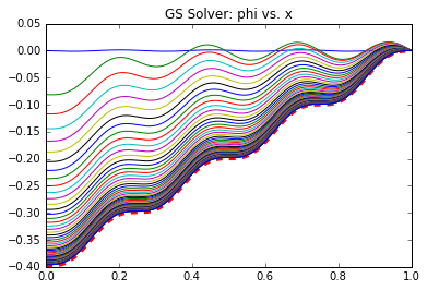
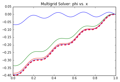
This also involved 5 operations but these occur only every R_freq iterations. Hence, the total number of iterations for the GS solver is (num_its*ni*5 + (num_its/R_freq)*5). This same GS scheme is used in the Multigrid solver to iterate \((\phi^n)^*\) and \(\epsilon_c\), with the caveat that the second iteration is on (ni/2) nodes. We additionally have operations to compute the residue and interpolate between meshes. Some of these operations could be optimized out but I kept them here for clarity. Comparing operation counts, we see that the MG needs a factor of 6.9 fewer operations that Gauss Seidel (1.6 million vs. 11.1 million)! Not bad at all. This result was obtained using only a single iteration to update \((\phi^n)^*\) (so only a single pass), and 50 iterations to approximate \(\epsilon_c\). These values were arrived at by trial and error so there may be better combinations out there. Figure 6 below plots the evolution of the solution \(\phi^n\) for the two solvers. The Gauss-Seidel data on left shows the solution every 250 iterations, while the Multigrid plot on right plots data after every 25 iterations on the fine level. We can clearly see the benefit of the Multigrid scheme: the number of iterations on the fine mesh, which contains more data points, is greatly reduced! The effect is even more pronounced in 2D and 3D where the number of unknowns reduces by a factor of 4 or 8 between each grid level. As a final note, most “production” multigrid solvers use additional levels of refinement. A common scheme is the “W”. It uses three grid levels 1,2,3 from the coarsest to the finest. We visit the grids like 3-2-1-2-1-2-3 which, if plotted, would give a W shape.
Code
Here is a snippet of the Multigrid solver
#multigrid solver
def MGsolve(phi,b):
    global eps_f, eps_c, R_f, R_c
    print("**** MULTIGRID SOLVE ****")
    ni = len(phi)
    ni_c = ni>>1    #divide by 2
    dx_c = 2*dx

    R_f = np.zeros(ni)
    R_c = np.zeros(ni_c)
    eps_c = np.zeros(ni_c)
    eps_f = np.zeros(ni)

    pl.figure()
    #plot analytical solution
    pl.plot(x,phi_true,LineWidth=4,color='red',LineStyle="dashed")
    pl.title('Multigrid Solver: phi vs. x')

    for it in range(10001):

        #number of steps to iterate at the finest level
        inner_its = 1

        #number of steps to iterate at the coarse level
        inner2_its = 50
        w = 1.4

        #1) perform one or more iterations on fine mesh
        for n in range(inner_its):
            phi[0] = phi[1]
            for i in range (1,ni-1):
                g = 0.5*(phi[i-1] + phi[i+1] - dx*dx*b[i])
                phi[i] = phi[i] + w*(g-phi[i])

        #2) compute residue on the fine mesh, R = A*phi - b
        for i in range(1,ni-1):
            R_f[i] = (phi[i-1]-2*phi[i]+phi[i+1])/(dx*dx) - b[i]
        R_f[0] = (phi[0] - phi[1])/dx    #neumann boundary
        R_f[-1] = phi[-1] - 0   #dirichlet boundary

        #2b) check for termination
        r_sum = 0
        for i in range(ni):
            r_sum += R_f[i]*R_f[i]
        norm = np.sqrt(r_sum)/ni
        if (norm<1e-4):
            print("Converged after %d iterations"%it)
            print("This is %d solution iterations on the fine mesh"%(it*inner_its))
            op_count_single = (inner_its*ni*5 + ni*5 + (ni>>1) +
                               inner2_its*(ni>>1)*5 + ni + ni)
            print("Operation count: %d"%(op_count_single*it))
            pl.plot(x,phi)
            return op_count_single*it
            break

        #3) restrict residue to the coarse mesh
        for i in range(2,ni-1,2):
            R_c[i>>1] = 0.25*(R_f[i-1] + 2*R_f[i] + R_f[i+1])
        R_c[0] = R_f[0]

        #4) perform few iteration of the correction vector on the coarse mesh
        eps_c[:] = 0
        for n in range(inner2_its):
            eps_c[0] = eps_c[1] + dx_c*R_c[0]
            for i in range(1,ni_c-1):
                g = 0.5*(eps_c[i-1] + eps_c[i+1] - dx_c*dx_c*R_c[i])
                eps_c[i] = eps_c[i] + w*(g-eps_c[i])

        #5) interpolate eps to fine mesh
        for i in range(1,ni-1):
            if (i%2==0):    #even nodes, overlapping coarse mesh
                eps_f[i] = eps_c[i>>1]
            else:
                eps_f[i] = 0.5*(eps_c[i>>1]+eps_c[(i>>1)+1])
            eps_f[0] = eps_c[0]

        #6) update solution on the fine mesh
        for i in range(0,ni-1):
            phi[i] = phi[i] - eps_f[i]

        if (it % int(25/inner_its) == 0):
            pl.plot(x,phi)

    return -1
Attachments
Source code: multigrid.py
You can speed up the multigrid further by doing a deeper v-cycle. So going from a fine mesh to a coarse mesh to an even coarser the operation count ratio went from
Operation count ratio (GS/MG): 6.91105
to
Operation count ratio (GS/MG): 82.2093
And the duration to solve the potential went from
5.609375 seconds for Gauss-Seidel
0.859375 seconds for MG with 1 level coarse grid V cycle
0.28125 secondss for MG with 2 levels coarse grid V cycle.
Here is the modified code for a 2 level coarse grid MultiGrid solver.
# -*- coding: utf-8 -*-
“””
Example 1D Multigrid solver
Written by Lubos Brieda for
https://www.particleincell.com/2018/multigrid-solver/
Modified by John Coady for 2 level MultiGrid V cycle for improved result.
Fri Mar 9 21:47:15 2018
“””
import numpy as np
import pylab as pl
import time
#standard GS+SOR solver
def GSsolve(phi,b):
print(“**** GS SOLVE ****”)
#plot for solution vector
fig_sol = pl.figure()
#plot analytical solution
pl.plot(x,phi_true,LineWidth=4,color=’red’,LineStyle=”dashed”)
pl.title(‘GS Solver: phi vs. x’)
#plot for error
fig_err = pl.figure()
pl.title(‘GS Solver: (phi-phi_true) vs. x’)
R_freq = 100 #how often should residue be computed
w = 1.4 #SOR acceleration factor
for it in range(100001):
phi[0] = phi[1] #neumann BC on x=0
for i in range (1,ni-1): #Dirichlet BC at last node so skipping
g = 0.5*(phi[i-1] + phi[i+1] – dx*dx*b[i])
phi[i] = phi[i] + w*(g-phi[i])
#compute residue to check for convergence
if (it%R_freq==0):
r_i = phi[1]-phi[0]
r_sum = r_i*r_i
for i in range (1, ni-1):
r_i = (phi[i-1]-2*phi[i]+phi[i+1])/(dx*dx) – b[i]
r_sum += r_i*r_i
norm = np.sqrt(r_sum)/ni
if (norm>1 #divide by 2
dx_2h = 2*dx
ni_4h = ni_2h>>1 #divide by 2
dx_4h = 2*dx_2h
R_h = np.zeros(ni_h)
R_2h = np.zeros(ni_2h)
R_4h = np.zeros(ni_4h)
eps_4h = np.zeros(ni_4h)
eps_2h = np.zeros(ni_2h)
eps_h = np.zeros(ni_h)
pl.figure()
#plot analytical solution
pl.plot(x,phi_true,LineWidth=4,color=’red’,LineStyle=”dashed”)
pl.title(‘Multigrid Solver: phi vs. x’)
for it in range(10001):
#number of steps to iterate at the finest level
inner_its = 1
#number of steps to iterate at the coarse level
inner2h_its = 5
inner4h_its = 50
w = 1.4
#1) perform one or more iterations on fine mesh
for n in range(inner_its):
phi[0] = phi[1]
for i in range (1,ni-1):
g = 0.5*(phi[i-1] + phi[i+1] – dx*dx*b[i])
phi[i] = phi[i] + w*(g-phi[i])
#2) compute residue on the fine mesh, R = A*phi – b
for i in range(1,ni-1):
R_h[i] = (phi[i-1]-2*phi[i]+phi[i+1])/(dx*dx) – b[i]
R_h[0] = (phi[0] – phi[1])/dx #neumann boundary
R_h[-1] = phi[-1] – 0 #dirichlet boundary
#2b) check for termination
r_sum = 0
for i in range(ni):
r_sum += R_h[i]*R_h[i]
norm = np.sqrt(r_sum)/ni_h
if (norm>1) +
inner2h_its*(ni_h>>1)*5 + ni_h + ni_h)
print(“Operation count: %d”%(op_count_single*it))
pl.plot(x,phi)
return op_count_single*it
break
#3) restrict residue to the 2h mesh
for i in range(2,ni_h-1,2):
R_2h[i>>1] = 0.25*(R_h[i-1] + 2*R_h[i] + R_h[i+1])
R_2h[0] = R_h[0]
#4) perform few iteration of the correction vector on the coarse mesh
eps_2h[:] = 0
for n in range(inner2h_its):
eps_2h[0] = eps_2h[1] + dx_2h*R_2h[0]
for i in range(1,ni_2h-1):
g = 0.5*(eps_2h[i-1] + eps_2h[i+1] – dx_2h*dx_2h*R_2h[i])
eps_2h[i] = eps_2h[i] + w*(g-eps_2h[i])
# Second V Restriction
#3a) restrict residue to the 4h mesh
for i in range(2,ni_2h-1,2):
R_4h[i>>1] = 0.25*(R_2h[i-1] + 2*R_2h[i] + R_2h[i+1])
R_4h[0] = R_2h[0]
#4a) perform few iteration of the correction vector on the coarse mesh
eps_4h[:] = 0
for n in range(inner4h_its):
eps_4h[0] = eps_4h[1] + dx_4h*R_4h[0]
for i in range(1,ni_4h-1):
g = 0.5*(eps_4h[i-1] + eps_4h[i+1] – dx_4h*dx_4h*R_4h[i])
eps_4h[i] = eps_4h[i] + w*(g-eps_4h[i])
#5a) interpolate eps to 2h mesh
for i in range(1,ni_2h-1):
if (i%2==0): #even nodes, overlapping coarse mesh
eps_2h[i] = eps_4h[i>>1]
else:
eps_2h[i] = 0.5*(eps_4h[i>>1]+eps_4h[(i>>1)+1])
eps_2h[0] = eps_4h[0]
#5) interpolate eps to fine mesh
for i in range(1,ni_h-1):
if (i%2==0): #even nodes, overlapping coarse mesh
eps_h[i] = eps_2h[i>>1]
else:
eps_h[i] = 0.5*(eps_2h[i>>1]+eps_2h[(i>>1)+1])
eps_h[0] = eps_2h[0]
#6) update solution on the fine mesh
for i in range(0,ni_h-1):
phi[i] = phi[i] – eps_h[i]
if (it % int(25/inner_its) == 0):
pl.plot(x,phi)
# print(“it: %d, norm: %g”%(it, norm))
return -1
ni = 128
#domain length and mesh spacing
L = 1
dx = L/(ni-1)
x = np.arange(ni)*dx
phi = np.ones(ni)*0
phi[0] = 0
phi[ni-1] = 0
phi_bk = np.zeros_like(phi)
phi_bk[:] = phi[:]
#set RHS
A = 10
k = 4
b = A*np.sin(k*2*np.pi*x/L)
#analytical solution
C1 = A/(k*2*np.pi/L)
C2 = – C1*L
phi_true = (-A*np.sin(k*2*np.pi*x/L)*(1/(k*2*np.pi/L))**2 + C1*x + C2)
pl.figure(1)
pl.title(‘Right Hand Side’)
pl.plot(x,b)
t = time.process_time()
#do some stuff
op_gs = GSsolve(phi,b)
elapsed_time = time.process_time() – t
print(“GS took : %g secs”, (elapsed_time))
t = time.process_time()
#reset solution
phi = phi_bk
op_mg = MGsolve(phi,b)
elapsed_time = time.process_time() – t
print(“MG took : %g secs”, (elapsed_time))
print(“Operation count ratio (GS/MG): %g”%(op_gs/op_mg))
You can try running these MultiGrid python example files online in the cloud here as Jupyter Notebooks.
https://mybinder.org/v2/gh/jcoady/MultiGrid/HEAD
There are 3 Jupyter Notebook files. The first one just executes a single level MultiGrid solver. The second notebook is a 2 level MultiGrid solver and the third one is a 3 level MultiGrid solver. Try running the code in each of the notebooks and compare the results. I also put the notebooks in a github repository here.
https://github.com/jcoady/MultiGrid
I updated the MultiGrid code further and improved the performance of the multigrid solver even more. There are 4 multigrid files with 1 V-cycle level, 2 V-cycle levels, 3 V-cycle levels and 4 V-cycle levels respectively. What I am seeing is that if there are more V-cycle levels then the multigrid code runs even faster to solve the problem. Here are the results that I am getting with
ni = 128
for 1 V-cycle level MultiGrid was 7.39054 times faster than Gauss-Seidel
for 2 V-cycle levels MultiGrid was 25.293 times faster than Gauss-Seidel
for 3 V-cycle levels MultiGrid was 38.7557 times faster than Gauss-Seidel
for 4 V-cycle levels MultiGrid was 54.4867 times faster than Gauss-Seidel
If I increased ni to 256 then I get the following results.
for 1 V-cycle level MultiGrid was 7.81608 times faster than Gauss-Seidel
for 2 V-cycle levels MultiGrid was 40.0115 times faster than Gauss-Seidel
for 3 V-cycle levels MultiGrid was 126.4 times faster than Gauss-Seidel
for 4 V-cycle levels MultiGrid was 254.213 times faster than Gauss-Seidel
You can try running these python codes for yourself online as Jupyter Notebooks at this link.
https://mybinder.org/v2/gh/jcoady/MultiGrid/HEAD
And the Jupyter Notebook files are located here on github.
https://github.com/jcoady/MultiGrid
Here is an MIT lecture on MultiGrid where these V-cycle concepts are explained starting around the 19 minute mark in the video.
https://ocw.mit.edu/courses/mathematics/18-086-mathematical-methods-for-engineers-ii-spring-2006/video-lectures/lecture-16-general-methods-for-sparse-systems/
I made a 3D version of the MultiGrid code in C++. The code can be found on github here.
https://github.com/jcoady/MultiGrid/tree/main/cpp
I used the 3D multigrid version to solve poisson equation for a 3D box with Dirichlet boundary conditions as shown in this video.
https://www.youtube.com/watch?v=4hSWZU4gjKs
The 3D multigrid solver was around 5 times faster than Gauss-Seidel solver but was about 10 times slower than the FFT solver for this problem.