Introduction to Vlasov Solvers

This is the first in a series of two posts that will first introduce you to Vlasov solvers and then to using Javascript WebGL to develop a GPU simulation running in your browser. Stay tuned, part two coming soon!

Boltzmann Equation

The objective of just about all plasma and gas-dynamics codes is simulating the evolution of one or more gas species given some initial conditions and a set of simple, first principle laws governing the motion and acceleration of the gas elements. Imagine that you could freeze all molecules in some small region for just long enough to somehow measure their x, y, and z velocities. Since the number of molecules is huge (there are over 10¹⁶ of them per cubic meter in a high quality “vacuum” chamber used for plasma propulsion testing), it may make more sense to create a histogram for each dimension. You then record how many molecules fall into each three-dimensional velocity bin. In the limit of the bins becoming infinitesimal, the result will be a continuous function for the count of molecules having some particular velocity components, \(N=f(u,v,w)\). (Alternatively, the function could be normalized so the result is the probability of finding such a molecule). The distribution you just computed is valid only for that particular spatial location and the current time. Thus, we also need to specify the location and the time to sample, giving you a function of seven variables, \(N=f(x,y,z,u,v,w,t)\). This is known as the velocity distribution function (or VDF for short).

Just as we have conservation laws for mass, momentum, and energy, there is a conservation law for the velocity distribution. It simply states that the total derivative of the VDF can only change through collisions,
$$\frac{df}{dt} = \left(\frac{\partial f}{\partial t}\right)_{col}$$
We can next rewrite the total derivative using the chain rule,
$$\frac{\partial f}{\partial t} + \frac{\partial f}{\partial x}\frac{\partial x}{\partial t} + \frac{\partial f}{\partial y}\frac{\partial y}{\partial t}+ \frac{\partial f}{\partial z}\frac{\partial z}{\partial t} + \frac{\partial f}{\partial u}\frac{\partial u}{\partial t} + \frac{\partial f}{\partial v}\frac{\partial v}{\partial t}+ \frac{\partial f}{\partial w}\frac{\partial w}{\partial t}= \left(\frac{\partial f}{\partial t}\right)_{col}$$
Now, \(\partial x/\partial t\) is just another way to write the x-component of velocity \(u\). Similarly, \(\partial u/\partial t = a_x\), the x-component of acceleration. With these substitutions, we obtain,
$$\frac{\partial f}{\partial t} + u\frac{\partial f}{\partial x} + v\frac{\partial f}{\partial y} + w\frac{\partial f}{\partial z} + a_x\frac{\partial f}{\partial u} + a_y\frac{\partial f}{\partial v}+ a_z\frac{\partial f}{\partial w} = \left(\frac{\partial f}{\partial t}\right)_{col}$$
The second, third, and fourth terms on the LHS can be further rewritten using vector notation by defining \(\mathbf{u}=u\mathbf{\hat{i}}+v\mathbf{\hat{j}}+w\mathbf{\hat{k}}\) and \(\nabla = (\partial/\partial x)\mathbf{\hat{i}} + (\partial/\partial y)\mathbf{\hat{j}} + (\partial/\partial z)\mathbf{\hat{k}}\), which is just the standard “spatial” gradient. This gives us
$$\frac{\partial f}{\partial t} + \mathbf{u}\cdot \nabla f + a_x\frac{\partial f}{\partial u} + a_y\frac{\partial f}{\partial v}+ a_z\frac{\partial f}{\partial w} = \left(\frac{\partial f}{\partial t}\right)_{col}$$
We can do something similar for the remaining components by defining a new type of a gradient operating on the velocity components, \(\nabla_u = (\partial/\partial u)\mathbf{\hat{i}} + (\partial/\partial v)\mathbf{\hat{j}} + (\partial/\partial w)\mathbf{\hat{k}}\). Utilizing Newton’s second law \(\mathbf{F}=m\mathbf{a}\), we can rewrite acceleration in terms of forces, giving us the final form,
$$\frac{\partial f}{\partial t} + \mathbf{u}\cdot \nabla f + \frac{\mathbf{F}}{m}\cdot \nabla_u f = \left(\frac{\partial f}{\partial t}\right)_{col}$$

This is known as the Boltzmann equation. Integrating it using standard methods from numerical analysis gives us a complete description of the gas at any spatial point at a future time. This sounds great, but there is a reason why Boltzmann solvers are relatively rare. Instead, you may be more familiar with plasma simulation methods based on the Particle in Cell (PIC) or Magnetohydrodynamics (MHD) methods. It all comes down to performance. Computers can’t store arbitrary continuous data, and thus we are forced to discretize the computational domain into cells. This is also done in PIC and MHD. But with Boltzmann solvers, we need to further subdivide each spatial cell into a three-dimensional velocity grid. This is the histogram alluded to before. Let’s consider an extremely crude 20x20x20 velocity space gridding. In each cell we thus need to allocate enough memory for 8,000 floats. With 4 bytes per float (using single precision), we need almost 32 kB (almost since 1kB = 1024B) per cell. Next couple this with another coarse 100x100x100 spatial mesh, and we see that a whopping 30 GB of RAM is needed for a single VDF! Numerical integration schemes will typically require a secondary buffer to compute temporary solutions, doubling the requirements. To make the problem worse, we generally need much finer velocity gridding, and our simulation will usually contain multiple species, each carrying their own VDF.

This is why methods such as MHD and PIC exist. With MHD (and its neutral gas counterpart CFD), we assume that the velocity distribution function has a certain shape that can be described by an analytical function. Specifically, we let
$$
f(u) = \frac{1}{\sqrt{\pi}v_{th}} \exp\left[\frac{-m(u-u_s)^2}{v_{th}^2}\right]
$$
where \(v_{th}=\sqrt{2kT_x/m}\). The huge benefit of this approach is that the entire VDF can be described with just 6 floats: the three stream velocity component \(u_s, v_s, w_s\) and the three corresponding temperatures. Often, we assume isotropic temperature leaving us with just a single temperature to worry about. Since the function is continuous, we actually obtain a more refined description of the complete VDF with just 4 floats than was accomplished previously with our 8,000 entry histogram. But the obvious downside is that some particular shape of the VDF had to be assumed. The above form is known as the Maxwellian distribution, and it describes the natural state molecules reach after a “sufficient” number of collisions. But in many rarefied gas simulations, there may not be enough collisions to guarantee this distribution. Therefore, kinetic methods such as PIC have been devised. With PIC, we use random numbers to select some sufficiently large number of velocity samples in each cell. We call these macroparticles, and use the equations of motion to advance their velocity and position. PIC allows us to resolve the VDF self-consistently. The downside is the noise associated with the stochastic sampling. PIC methods are thus more suitable to steady-state computations where the results can be averaged over a large number of iterations.

One-Dimensional Vlasov Solver

But one area where Boltzmann solvers can be applied efficiently is in one-dimensional problems. The rest of this article will show you how to develop a one-dimensional solver for the Vlasov equation, which is a special form of the Boltzmann equation in which collisions (the term on the RHS) is ignored. We will use the approach used by Cheng and Knorr in their integral 1975 J. Computational Physics paper “Integration of the Vlasov Equation in Configuration Space” (pdf) and apply the code to the following equation
$$\frac{\partial}{\partial t}f(x,u,t) + u\frac{\partial}{\partial x}f(x,u,t) – E(x,t)\frac{\partial}{\partial u}f(x,u,t)=0 $$
This is the normalized 1-D Vlasov equation for an electron with charge \(q=-1\) and mass \(m=1\). The authors then solve this equation by splitting the integration into two parts,
$$
\begin{align}
\frac{\partial f}{\partial t} + u\frac{\partial f}{\partial x} &= 0 \qquad(1)\\
\frac{\partial f}{\partial t} – E(x,t)\frac{\partial f}{\partial u} &=0 \qquad(2)
\end{align}
$$

Equation (1) above can be rewritten using forward differencing as
$$ \frac{f^{k+1}(x,u)-f^{k}(x,u)}{\Delta t} = -v\frac{\partial f^k}{\partial x}$$
or
$$f^{k+1} (x,u) = f^k(x,u) – v\frac{\partial f^k}{\partial x}(x,u)\frac{\Delta t}{2}$$
This may not be obvious at first, but the term on the RHS is actually a shift of the distribution function in the spatial direction. This is because
$$
f-\frac{\partial f}{\partial x}u\Delta t = f-\frac{\partial f}{\partial x}\frac{\Delta x}{\Delta t}\Delta t=f-\frac{\partial f}{\partial x}\Delta x
$$
and we can write \( f^{k+1}(x,u) = f^k(x-u\Delta t/2,u) \)

In the paper, the authors show that the electric field in (2) needs to be evaluated at the half-time step for stability. We then end up with the following three steps:

1. Integrate equation (1) through half time step. Using PIC analogy, this is similar to using velocity from the previous time step to compute positions at time (k+0.5).
2. Compute the electric field using charge density at time (k+0.5) and use it advance equation (2) through a whole time step. This gives us the new velocity at time (k+1).
3. Perform the second half-step integration of (1). Again using the particle analogy, this gives us the new position at time (k+1) using the velocity at (k+1).

We write these steps using temporary arrays:
$$
\begin{align}
f^*(x,u) &= f^k(x-u\Delta t /2,v)\\
E &= E(f^*) \\
f^{**}(x,u) &= f^*(x,u+E(x,t)\Delta t)\\
f^{k+1}(x,u) &= f^{**}(x-u\Delta t/2,v)
\end{align}
$$
The above equation is written for the normalized electrons, in general, you would have \(-F(x,t)/m\) on the RHS instead of the electric field. The second equation is meant to indicate that we use \(f^*\) to compute the new values for the electric field.

Implementation

Data

We will now see how to actually implement the above equations. Our computational domain is a two-dimensional mesh, but the “j” component is not “y” but the velocity. Therefore, the value stored at some (i,j) grid node corresponds to the value of the distribution function at the i-th x position and the j-th velocity. We let x go from zero to some length L. The velocity discretization needs to capture particles moving in both positive and negative direction, and thus the velocity goes from (-v_max) to (+v_max). This is sketched in Figure 1 below.

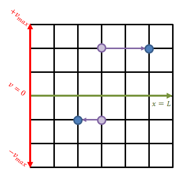
The green line divides the velocity space into the positive and negative sub-space. Each mesh node stores the value of the distribution function at that specific spatial position (x-axis) and velocity (y-axis). In a way, we can imagine that at each grid node we have a macroparticle with specific weight corresponding to the value of the VDF. All macroparticles located above the green line have positive velocity and thus they move to the right. The speed increases with the distance from the centerline and thus a “particle” located two cells above will move greater horizontal distance than a particle located only unit cell away. This is visualized in the figure.

We will need arrays to store f, fs, and fss. We really need just two arrays since all integration steps use one array to compute a new one (such as f->fs). We can then overwrite the “old” array with the “new” value and use the old array to now compute the next step. But here for clarity all three are kept. We will also need memory to store charge density and electric field. These are one-dimensional quantities varying only with x. The example code uses a helper function newAndClear to allocated 1D or 2D array and initialize its values to zero.

double **f = newAndClear(ni,nj); //f
double **fs = newAndClear(ni,nj); //fs
double **fss = newAndClear(ni,nj); //fss
double *ne = newAndClear(ni);	//number density
double *b = newAndClear(ni);	//Poisson solver RHS, -rho=(ne-1) since ni=1 is assumed
double *E = newAndClear(ni);	//electric field
double *phi = newAndClear(ni);	//potential

Initial Conditions

The next thing we need to do after allocating the memory is to load some initial distribution function. We assume that electrons are Maxwellian, and load a normalized variant,
$$f(u) = \frac{1}{\sqrt{\pi u_{th}^2}}\exp\left[-\frac{(u-u_d)^2}{u_{th}^2}\right]$$

For instance, we could do the following

//set initial distribution
for (int i=0;i<ni;i++)
    for (int j=0;j<nj;j++)
    {
	double x = world.getX(i);
	double v = world.getV(j);
 
	double vth2 = 0.01+(x/world.L)*(2-0.01);
	double vs = 1.5;
	f[i][j] = 1.0/sqrt(vth2*pi)*exp(-(v-vs)*(v-vs)/vth2);
    }

This code loads a VDF with uniform streaming velocity 1.5, but thermal velocity (and thus temperature) linearly increasing from 0.01 on the left edge to 2 on the right one. In other words, we have some gas that is on average moving at 1.5 units per second but is getting hotter towards the right edge.

Main Loop

All that is left next we adding the main loop to implement the three step method of Cheng and Knorr from above:

for (it=0;it<=2000;it++)
{
	if (it%5==0)
		saveVTK(it,world,scalars2D,scalars1D);
 
	//compute f*
	for (int i=0;i<ni;i++)
		for (int j=0;j<nj;j++)
		{
			double v = world.getV(j);
			double x = world.getX(i);			
			fs[i][j] = world.interp(f,x-v*0.5*dt,v);								
		}
	}
 
	//compute f**
	for (int i=0;i<ni;i++)
		for(int j=0;j<nj;j++)
		{
			double v = world.getV(j);
			double x = world.getX(i);
			fss[i][j] = world.interp(fs,x,v+E[i]*dt);				
		}
 
	//compute f(n+1)
	for (int i=0;i<ni;i++)
		for(int j=0;j<nj;j++)
		{
			double v = world.getV(j);
			double x = world.getX(i);
			f[i][j] = world.interp(fss,x-v*0.5*dt,v);
		}				
}

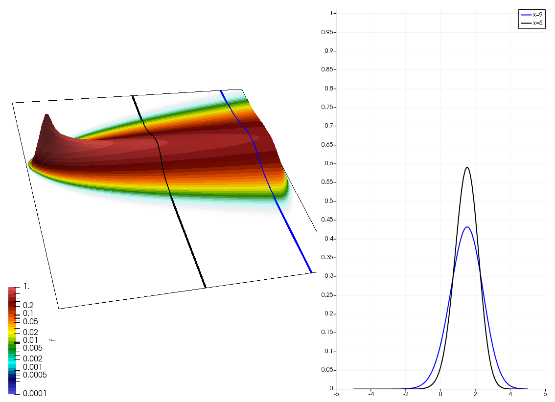
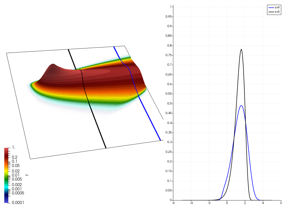
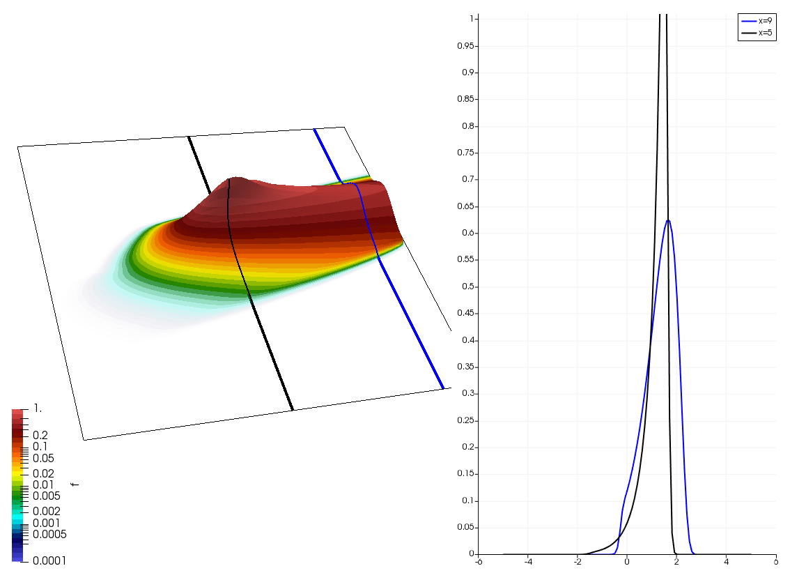
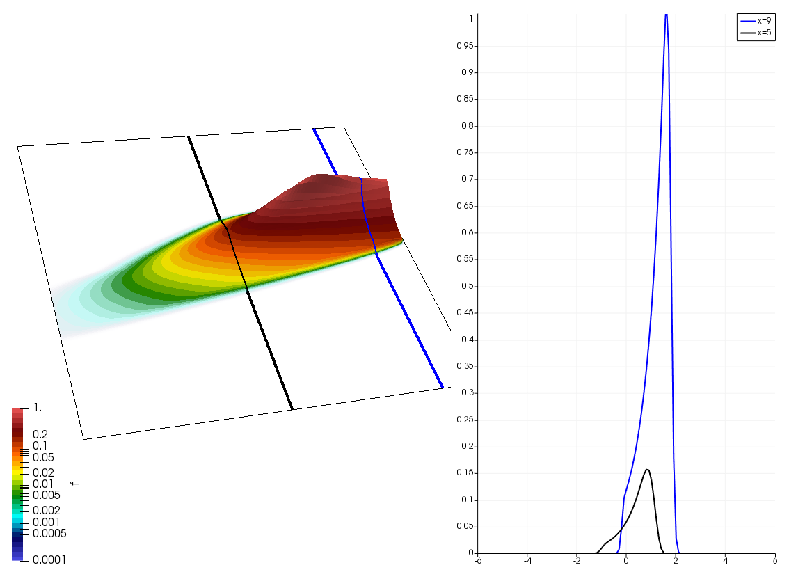
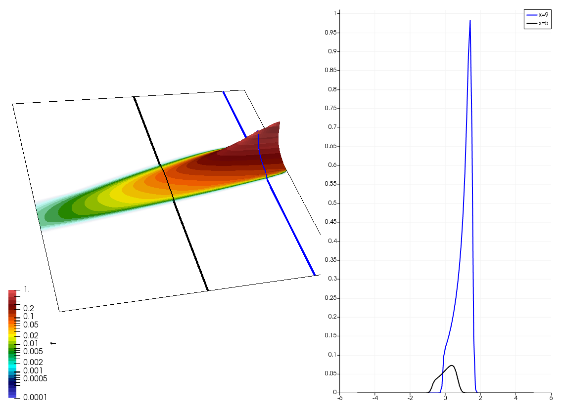
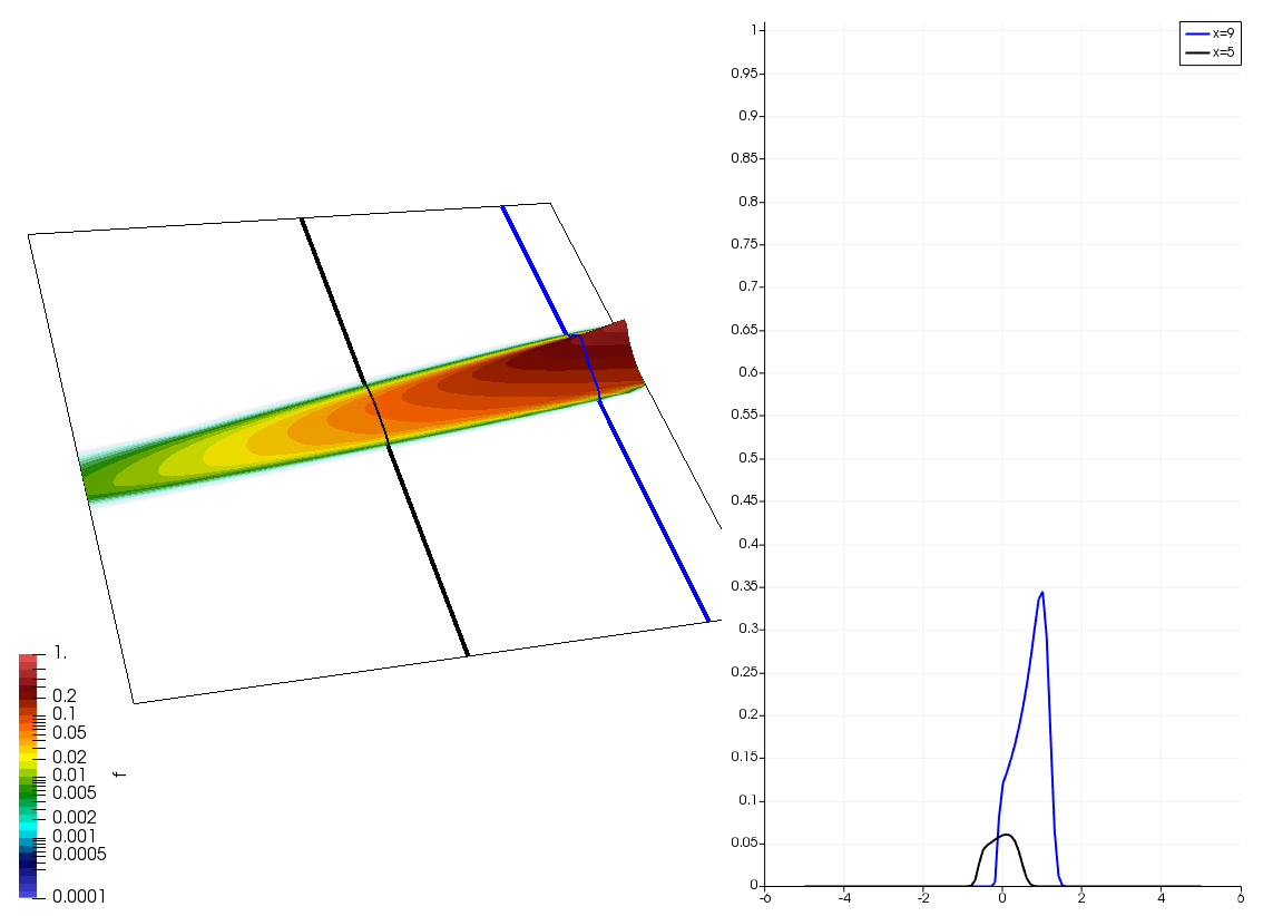
There really isn’t a lot to it! The code outputs the distribution function after every 5th time step and we can use Paraview to visualize the results. This is shown in Figure 2 below, where I ended up using the “Warp by Scalar” filter to give the plots some depth. The subplots visualize the VDF along two slices. These line plots may make it more obvious that we are indeed dealing with a Maxwellian VDF as the familiar bell curve shape is quite apparent. Majority of the population has \(u>0\) and hence the population moves to the right. We are running with open boundaries, and thus any gas leaving through the right edge is lost. We can see this in the blue slice by observing how to the VDF starts getting depleted from the right side (faster velocity). There is also a small population with negative velocities. These fluid parcels move to the left. But since their velocity magnitude is smaller than the initial streaming velocity, they continue to linger long after the bulk of the population left the computational domain.

Adding Electric Field

The above code is not complete, since it doesn’t include the self-consistent electric field computation. As we all know from basic plasma physics, in electrostatic plasma simulations, we obtain the electric field from \(E_x = -\partial \phi/\partial x\). Plasma potential is computed from Poisson’s equation, which in 1D is
$$\frac{\partial^2\phi}{\partial x^2} = \frac{e(n_e-Z_in_i)}{\epsilon_0}$$
Our code actually solves the normalized version:
$$\frac{\partial^2\phi}{\partial x^2} = n_e-1$$
Clearly, we need to somehow compute the electron number density at each spatial grid node. Number density is simply the number of molecules divided by the cell volume. Since the VDF gives us the number of molecules with some particular velocity, we can get the total particle count by integrating the VDF over all velocities,
$$N=\int_{-\infty}^{+\infty}f(u)du$$
We assume that the cell volume is unity and hence this integral gives us the number density. This integration is performed in the code with the trapezoid scheme,

//compute number density by integrating f with the trapezoidal rule		
for (int i=0;i<ni;i++)
{
	ne[i] = 0;
	for (int j=0;j<nj-1;j++)
		ne[i]+=0.5*(fs[i][j+1]+fs[i][j])*dv;
}

We then use any regular old Poisson solver, such as the 1D Gauss-Seidel scheme used previously in the PIC Fundamentals course. Note that periodic systems like this one can also be solved using Fourier Transforms.

Interpolation

The above code used an interp function to evaluate \(f(x,v)\) at arbitrary points that may not correspond to grid nodes. The code in the example uses the linear area-weighted scheme familiar to you all from PIC Fundamentals. While this method is ok for this introductory example, it is too diffusive to be used in real Vlasov solvers. The issue is that since the VDF typically decays rapidly away from the peak, linear weighing may over-estimate the number of fast moving molecules, leading to artificial diffusion. This interpolation function is defined as a method in a World object. It support both periodic and open boundaries in x.

//linear interpolation: a higher order scheme needed!
double interp(double **f, double x, double v)
{
	double fi = (x-0)/dx;
	double fj = (v-(-v_max))/dv;		
 
	//periodic boundaries in i
	if (periodic)
	{
		if (fi<0) fi+=ni-1;		//-0.5 becomes ni-1.5, which is valid since i=0=ni-1
		if (fi>ni-1) fi-=ni-1;
	}
	else if (fi<0 || fi>=ni-1) return 0;
 
	//return zero if velocity less or more than limits
	if (fj<0 || fj>=nj-1) return 0;
 
	int i = (int)fi;
	int j = (int)fj;
	double di = fi-i;
	double dj = fj-j;
 
	double val = (1-di)*(1-dj)*f[i][j];
	if (i<ni-1) val+=(di)*(1-dj)*f[i+1][j];
	if (j<nj-1) val+=(1-di)*(dj)*f[i][j+1];
	if (i<ni-1 && j<nj-1) val+=(di)*(dj)*f[i+1][j+1];
	return val;		
}

Two-Stream Instability

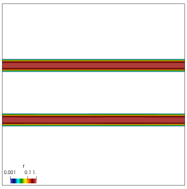
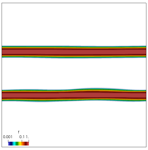
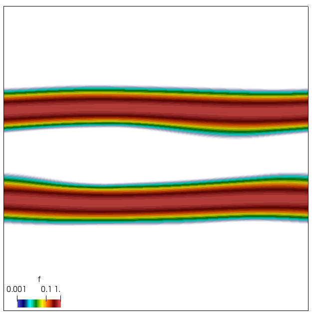
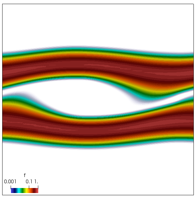
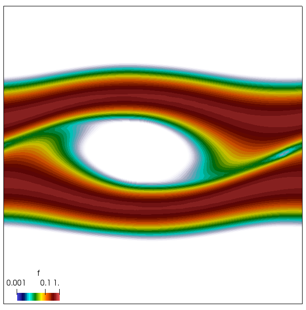
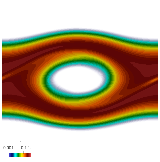
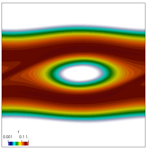
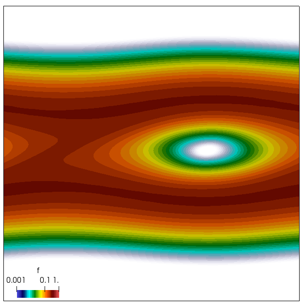
We now have all pieces to run a more interesting example. This setup was actually motivated by students of Andrei Smolyakov at University of Saskatchewan’s Theoretical Plasma Physics Group. The above example was used to introduce Vlasov solvers in my Fluids course, and for a homework assignment, I asked the students to write a code to simulate Landau Damping. Dr. Smolyakov students went beyond and wrote a code to simulate two stream instability. To run this, we simply modify the initial injection scheme to load two cold beams drifting in opposite directions. One of the beams (the one moving in the negative direction in my example) is also given small sinusoidal oscillations in density. This small noise is needed to induce some initial electric field that will cause the two populations to start interacting with each other. In PIC simulations (like this Javascript version), this field would eventually arise on its own from the noise inherent in all particle codes. But here it is better to introduce it explicitly otherwise you may need to wait for a very long time for anything interesting to happen!

//set initial distribution
for (int i=0;i<ni;i++)
	for (int j=0;j<nj;j++)
	{
		double x = world.getX(i);
		double v = world.getV(j);			
 
		double vth2 = 0.02;
		double vs1 = 1.6;
		double vs2 = -1.4;
		f[i][j] = 0.5/sqrt(vth2*pi)*exp(-(v-vs1)*(v-vs1)/vth2);
		f[i][j] += 0.5/sqrt(vth2*pi)*exp(-(v-vs2)*(v-vs2)/vth2)*(1+0.01*cos(3*pi*x/world.L));
	}

We also make our world periodic by setting world.periodic=true; and we also add a call to world.applyBC() after each VDF field is updated. This function simply makes the values on the left and right edges identical. The code was run with time step dt=1/8.0. Example results are shown below. This demo simulates two electron beams interacting with each other in a domain containing neutralizing ion background. The numerical diffusion introduced by the linear interpolation operator is quite apparent if you run the code longer. The vortex closes up rapidly, but stays open in the PIC simulation.

Code

And that’s all for today. The follow up article will show you how to write a version of this code that runs in your browser. Don’t forget to sign up for my plasma simulation courses if you want to learn more. Use g++ -std=c++11 -O2 vlasov.cpp to compile the code.
Code: vlasov.cpp