Computing pi with CPUs, GPUs, threads, MPI, Javascript, Arduino, and FPGAs

This year, for “pi day” (March 14th), I figured I’ll post a short article demonstrating how to estimate the value of π using different computer architectures. This topic is somewhat in line with the ASTE-499 Applied Scientific Computing Course I am currently teaching at USC’s Astronautical Engineering Department. The goal of that course is to provide students with the necessary computational background needed to tackle real computational projects.
Table of Contents
- Theory
- Serial C++
- Multithreaded C++
- MPI
- CUDA
- Javascript with Canvas
- Javascript with WebGL
- Arduino microcontroller
- FPGA
Theory
A simple way to estimate the value of π is from the area ratio between a unit circle and the enclosing unit square (or in this case, a unit quarter circle). We have the following:
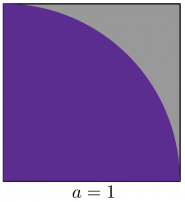
The ratio of areas is
\[
\frac{A_{qc}}{A_s} = \frac{\pi a^2/4}{a^2}=\frac{\pi}{4}
\]
Therefore, if we could estimate the two areas, we can use their ratio to obtain a value of π. Turns out, there is a very simple way to do so. We can simply select a large number of uniformly distributed points within the square, \(x\in[0,a], \; y\in[0,a]\). For each point, we determine if it is in the circle, \(\sqrt{x^2 + y^2}\le a^2\). The fraction of points inside to the total number of points is identical to the area ratio between the circle and the square. Therefore,
\[
\pi \approx 4\frac{N_{in}}{N_{tot}}
\]
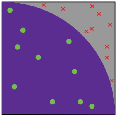
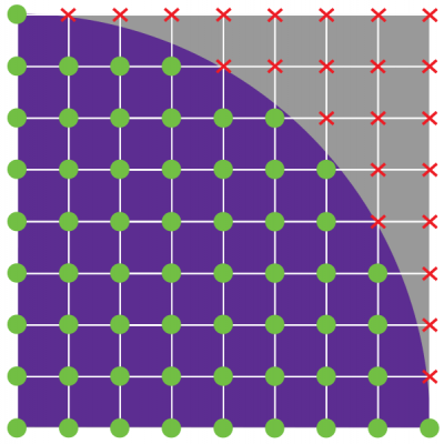
There are two ways to select the points. We can either use a stochastic (i.e. random) sampling, or we can utilize a fine uniform grid. The first approach is analogous to throwing a dart at the square and checking if it lands inside the circle. Obviously we need a huge number of darts (random samples) to get a good approximation of the ratio. With the second approach, we need to use a very fine gridding to get a large number of points.
Serial C++
The simplest way to implement this algorithm is with a serial code running on the CPU (the computer processor).
#include <iostream>
#include <iomanip>
#include <random>
#include <math.h>

using namespace std;

// object for sampling random numbers
class Rnd {
public:
  //constructor: set initial random seed and distribution limits
  Rnd(): mt_gen{std::random_device()()}, rnd_dist{0,1.0} {}
  double operator() () {return rnd_dist(mt_gen);}

protected:
  std::mt19937 mt_gen;	    //random number generator
  std::uniform_real_distribution<double> rnd_dist;  //uniform distribution
};

Rnd rnd;		// instantiate the Rnd object

int main() {
  size_t N_total = 1000000;
  size_t N_in = 0;

  for (size_t s=0;s<N_total;s++) {
    double x = rnd();        // pick random x in [0,1)
    double y = rnd();        // pick random y in [0,1)
    if (x*x+y*y<=1) N_in++;  // increment counter if inside the circle
  }

  double pi = 4*N_in/(double)N_total;  // cast to double to perform floating point division
  double error = 100*abs(pi/acos(-1.0)-1); // (our-real)/real
  cout<<"Using "<<N_total<<" samples, pi is "<<pi<<" ("<<setprecision(2)<<error<<"% error)"<<endl;

  return 0;
}
Source: pi-serial.cpp
Compiling and running the code few times we get
$ g++ pi-serial.cpp -o pi-serial
$ ./pi-serial
Using 1000000 samples, pi is 3.1404 (0.038% error)
$ ./pi-serial
Using 1000000 samples, pi is 3.138 (0.11% error)
$ ./pi-serial
Using 1000000 samples, pi is 3.138 (0.11% error)
Alright, the code is definitely working although the estimate is not the greatest. Increasing the number of samples to 10 million, we obtain an improved estimate.
$ Using 10000000 samples, pi is 3.14132 (0.0087% error)
Multithreaded C++
Of course, using more samples also takes longer. For this reason, this algorithm is the common “Hello World” example for parallel computing. One way to speed it up is by utilizing the multiple cores present on all modern CPUs (for instance, the Intel i7-8700 chip in my desktop workstation has 6 physical cores). A serial code as the one above uses only one core at a time. We can take advantage of multiple cores by splitting the computation into multiple threads. Each thread is a block of code that runs in parallel with other threads. Let’s say we want to run the computation with 4,000 samples. Instead of having one core check all 4,000 points, we can have 4 cores check 1,000 points each. We then simply compute the combined ratio from
\[
\frac{N_{qc}}{N_{total}} = \sum_i^{n_{threads}} \left.\frac{N_{qc}}{N_{total}}\right|_i
\]
Modern C++ (C++11) makes launching threads very easy. We simply create an object of type thread. It is important to realize that after the thread is launched, the main thread continues to run. Without any precautions, the main program may terminate before the worker threads had a chance to complete their computation. We thus need to wait for completion using join. This command blocks until the thread is done.
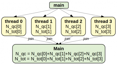
Another very important caveat to keep in mind is that code in parallel has access to the same memory. It is crucial to avoid having multiple threads write to the same memory location. This leads to a race condition where the result can vary based on which threads gets to it first. It is OK for multiple threads to read the same data, but any stored results need to be saved into a local buffer. The main thread then performs the final reduction. The overall algorithm looks like this:
The resulting code is below:
#include <iostream>
#include <iomanip>
#include <random>
#include <chrono>
#include <thread>
#include <vector>

using namespace std;

// object for sampling random numbers
class Rnd {
/* ... */

vector<Rnd> rnds;		// instantiate array of Rnd objects

// function to launch in parallel, we could alternatively define a class
// result is stored in N_in[thread_id]
void Worker(int thread_id, size_t N_total, size_t *N_ins) {
  // set references to thread-specific items
  size_t &N_in = N_ins[thread_id];	// result
  Rnd &rnd = rnds[thread_id];	        // our dedicated generator
  N_in = 0;
  for (size_t s=0;s<N_total;s++) {
    double x = rnd();
    double y = rnd();
    if (x*x+y*y<=1) N_in++;
  }
}

int main(int num_args, char**args) {
  // get maximum number of supported concurrent threads
  int num_threads = thread::hardware_concurrency();
  if (num_args>1) num_threads = atoi(args[1]); // get from command line

  // generate an array of random number generators
  rnds.resize(num_threads);

  // grab starting time
  auto time_start = chrono::high_resolution_clock::now();

  size_t N_goal = 100000000;
  size_t N_total = 0;

  // allocate memory for results
  size_t *N_in_arr = new size_t[num_threads];

  // container to store thread objects
  vector<thread> threads;

  // create threads
  for (int i=0;i<num_threads;i++) {
     size_t N_per_thread =  N_goal / num_threads;
     // correct on last one to get the correct total
     if (i==num_threads-1) N_per_thread = N_goal - (N_per_thread*(num_threads-1));
     N_total += N_per_thread;

     // launch Worker(i,N_per_thread,N_in_arr) in parallel
     threads.emplace_back(Worker,i,N_per_thread,N_in_arr);
  }

  // wait for workers to finish
  for (thread &th:threads)
   th.join();

  // sum up thread computed results
  size_t N_in = 0;
  for (int i=0;i<num_threads;i++) {
     N_in += N_in_arr[i];
  }

  auto time_now = chrono::high_resolution_clock::now();
  chrono::duration<double> time_delta = time_now-time_start;

  double pi = 4*N_in/(double)N_total;  // cast to double to perform floating point division
  cout<<"Using "<<N_total<<" samples and "<<num_threads<<" threads, pi is "<<pi
      <<" in "<<setprecision(3)<<time_delta.count()<<" seconds"<<endl;

  delete[] N_in_arr;
  return 0;
}
Source: pi-threads.cpp
The main difference from the serial version is that the computation has been moved to a Worker function. We launch this function in parallel by creating a new object of type thread. The constructor for std::thread requires any function-like (functor) object that can be called as Object(arg0, arg1, arg2, ...). These (optional) arguments can also be passed in to the thread constructor. For simplicity, here we use a regular function, and use an array of N_in[] to store the computed results. Alternatively, we could use a class with an overloaded operator() but that leads to a slightly more complex code. The reason for storing the threads in a vector is so that we can subsequently call join() to wait for the worker code to finish. The main function then sums up the values in N_in[] to get the total. Also, each worker is given the number of samples to check. Since the total desired number may not be evenly divisible by the number of threads, we update the count on the last thread to make sure we get the correct total. The number of threads is obtained from hardware_concurency() function but can be overridden by a command line argument. This default value represents the number of logical cores the CPU supports. This will typically be twice the number of actual hardware cores.
One other change you may have noticed is that we are using an array of random number geneators, vector
Compiling and running the code, we obtain
$ g++ -O2 pi-threads.cpp -o pi-threads -lpthread
$ ./pi-threads
Using 100000000 samples and 12 threads, pi is 3.14186 in 0.962 seconds
$ ./pi-threads 1
Using 100000000 samples and 1 threads, pi is 3.14156 in 3.02 seconds
$ ./pi-threads 4
Using 100000000 samples and 4 threads, pi is 3.14175 in 1.79 seconds
$ ./pi-threads 6
Using 100000000 samples and 6 threads, pi is 3.14159 in 1.24 seconds
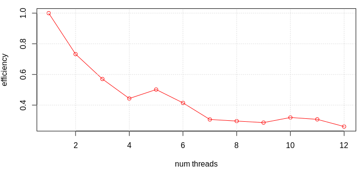
We can also record the run times and compute the parallel efficiency from
\[
k_{n} = \frac{t_1}{nt_n}
\]
times. We can then generate a plot in R using
> a<-1:12
> b<-c(2.96,2.02,1.73,1.67,1.2,1.19,1.38,1.25,1.15,0.927,0.876,0.948)
> plot(a,b[1]/(b*a),type="o",xlab="num threads",ylab="efficiency", col="red")
> grid()
As can be seen from Figure 4, parallel efficiency significantly decreases with more than 6 cores. This is because even though concurrent_threads returns 12 on my system, the CPU contains only 6 physical hardware cores.
C++ with MPI
The main downside of multithreading is that we are limited to the number of the relatively few computational cores available on a single CPU. The way to get around this is to split up the computation among multiple physical computers. The Message Passing Interface (MPI) is a library that allows different processes to communicate with each other. This communication happens primarily over the network, but MPI also supports multiple processes on the same physical computer.
MPI, by itself, does not perform any parallelization of the code. It only gives us the means to accomplish inter-process communication, but it is up to us to decide how to distribute the work load. Each process is assigned a unique rank and also knows the total number of processes. From this information, the process can compute the number of samples that it should check. Alternatively, in field solvers or PIC simulations, we may want to use this information to decide which section of the domain to check, in a process known as domain decomposition.
#include <iostream>
#include <iomanip>
#include <random>
#include <chrono>
#include <thread>
#include <sstream>
#include <mpi.h>

using namespace std;

// object for sampling random numbers
class Rnd {
/* ... */
};

Rnd rnd;		// instantiate an Rnd object

int main(int num_args, char**args) {
  MPI_Init(&num_args, &args);    // initialize MPI

  // grab starting time
  auto time_start = chrono::high_resolution_clock::now();

  // figure out what rank I am and the total number of processes
  int mpi_rank, mpi_size;
  MPI_Comm_rank(MPI_COMM_WORLD,&mpi_rank);
  MPI_Comm_size(MPI_COMM_WORLD,&mpi_size);

  // write to a stringstream first to prevent garbled output
  stringstream ss;
  ss<<"I am "<<mpi_rank<<" of "<<mpi_size<<endl;
  cout<<ss.str();

  // figure out how many samples I should process
  unsigned N_goal = 100000000;
  unsigned N_tot =  N_goal / mpi_size;

  // correct on last rank to get the correct total
  if (mpi_rank == mpi_size-1) N_tot = N_goal - (N_tot*(mpi_size-1));

  // perform the computation
  unsigned N_in = 0;
  for (size_t s=0;s<N_tot;s++) {
     double x = rnd();
     double y = rnd();
     if (x*x+y*y<=1) N_in++;
  }

  // sum up N_in and N_tot across all ranks and send the sum to rank 0
  unsigned N_tot_glob;
  unsigned N_in_glob;
  MPI_Reduce(&N_in,&N_in_glob,1,MPI_UNSIGNED,MPI_SUM,0,MPI_COMM_WORLD);
  MPI_Reduce(&N_tot,&N_tot_glob,1,MPI_UNSIGNED,MPI_SUM,0,MPI_COMM_WORLD);

  auto time_now = chrono::high_resolution_clock::now();
  chrono::duration<double> time_delta = time_now-time_start;

  // compute pi and show the result on rank 0 (root) using the global data
  if (mpi_rank==0) {
    double pi = 4*N_in_glob/(double)N_tot_glob;
    stringstream ss;
    ss<<"Using "<<N_tot_glob<<" samples and "<<mpi_size<<" processes, pi is "<<pi
      <<" in "<<setprecision(3)<<time_delta.count()<<" seconds"<<endl;
    cout<<ss.str();
  }

  MPI_Finalize();     // indicate clean exit
  return 0;
}
Source: pi-mpi.cpp
Each MPI process needs to call MPI_Init at start and MPI_Finalize at the end to indicate normal (in other words, not crashed) exit. We then call MPI_Comm_rank and MPI_Comm_size functions to get our rank and the total number of processes in the given communicator. MPI processes can be grouped into multiple communicators that can be used to cluster workers into separate task groups. There is always one global communicator available called MPI_COMM_WORLD.
These two functions thus return the global rank and the global size. For debugging, I also included code to print out each applications rank and size. In order to avoid garbled output where multiple processes are writing to the same screen line at the same time, we first write to a stringstream and then parse out the entire stream at once.
We then calculate how many samples to check, using the same formula that was used in the multithreaded version. The local data then needs to be collected (summed up) across all ranks to obtain the total number of good samples. This is accomplished here using the MPI_Reduce function. It is important that all ranks call this function with their local value, otherwise we get a deadlock. The specified operation (in this case MPI_SUM) is then applied and the result is stored at the address &N_in_glob
address but only on the specified rank (0 on this case). A similar MPI_Allreduce function distributes the reduced data
to all processes. In the case of large data, this could lead to unecessary network traffic if the other processes don’t actually need it. The root rank (rank=0) that received the reduced data then performs the final computation and also prints the output to the screen.
We compile this code using mpic++. This is basically just a wrapper on top of g++ that passes in all the appropriate header and library paths. We can use all standard g++ options such -O2. We launch the program using mpirun with -np argument specifying the number of processes to launch. On a proper cluster, you would also specify a hosts file that provides the IP address (or domain names) for the nodes to run the program on. This is something that should already be set up for you on whatever cluster you have access to. Otherwise, the code runs locally. This ends up being somewhat analogous to the multithreaded version with the exception that we now have several unique programs that cannot access each other’s memory space.
$ mpic++ -O2 pi-mpi.cpp -o pi-mpi
$ mpirun -np 4 ./pi-mpi
I am 0 of 4
I am 1 of 4
I am 2 of 4
I am 3 of 4
Using 100000000 samples and 4 processes, pi is 3.1416 in 0.789 seconds
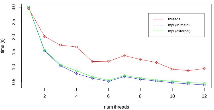
I next ran the code locally on my 6-core CPU workstation and again collected the run times. Here I collected both the value shown on the screen, coming from the different between time_now and time_start, but I also saved data from
$ /usr/bin/time -f "%e" mpirun -np XX ./pi-mpi
in order to capture the start up time. Interestingly, even including the start up time, the MPI version is noticeably faster than the multithreaded one. I wonder if the CPU prioritized multiple processes over multiple threads from the same process?
CUDA GPU
But wait, there is more! Modern computers often contain a graphics card or a GPU. GPUs are basically vector computers optimized for performing the same operation on different data in parallel (single instruction, multiple data, or SIMD). Consider vector addition,
for (int i=0;i<N;i++) c[i]=a[i]+b[i];
There is no need to compute c[0]=a[0]+b[0] before moving on to 1, and 2, and so on as is the case here. On a 100 core vector computer, we can instead perform the computation c[0:99]=a[0:99]+b[0:99] concurrently. This is what GPUs excel at. The actual coding is achieved using either OpenCL (general) or CUDA (for NVIDIA cards). We use CUDA here just because I am more familiar with it. CUDA is an extension to the C++ programming language that includes few additional keywords for creating kernel __global__ functions that run on the GPU (or the device), and for launching them. It also includes functions for allocating memory on the card and transferring it back to the CPU (called the host).
It is possible to sample random numbers on the GPU, but here we demonstrate the alternative non-stochastic approach shown by the right plot in Figure 2. We effectively generate a N*N grid and use the GPU threads to compute whether each grid node point is inside or out. We then sum up the number of internal points. We also do this summation on the GPU to both utilize the computational power but to also reduce the amount of memory needed to be transferred back to the CPU. The CPU-GPU memory transfer is a major bottleneck in GPU codes and hence it is the best to transfer as little data as possible.
CUDA allows us to launch threads as a grid of blocks each containing some grid of threads. The threads within the same block have access to fast shared memory. For this reason, we perform the computation using 16×16 thread blocks. Each thread is given access to several predefined dim3-type variables that can be used to figure out the thread and block indexes. The actual node index on the global grid is
\[
i = blockIdx.x*blockDim.x + threadIdx.x\\
j = blockIdx.y*blockDim.y + threadIdx.y
\]
In our case here, blockDim will be 16 and the threadIdx will be some number from 0 to 15. Also, there are total of 16*16=256 threads in a block. We allocate a shared boolean array, and let each thread set on item. I made the array one-dimensional, and use
\[
u = threadIdx.y*blockDim.x + threadIdx.x
\]
to compute a one-dimensional index. This is the same \(u=j\cdot ni+i\) flattening scheme we use in our plasma simulations.
The first thread in each block (thread with u=0) then loops over the array once all threads have finished and counts how many “ins” we have. This count is stored in a block_counts array located in GPU global memory. This is the main RAM on the GPU. It is slower than the block shared memory, which is why we try to utilize shared memory first. We again use a flattening
scheme to compute a one-dimensional index for each block per
\[
u_{block}= blockIdx.y*gridDim.x+blockIdx.x
\]
The memory for this array is allocated using cudaMalloc.
This is where the flagKernel ends. At this point, we have an array of num_blocks integers on the GPU. We could at this point transfer this array to the CPU and have the CPU perform the final sum. But to reduce the amount of data to be transferred, we perform this reduction using another GPU function addKernel. We run this kernel serially (just a single GPU thread) for simplicity which introduces some inefficiency. The computed sum is stored into another global memory variable. We then finally transfer the contents of this variable (the total N_in) from the GPU to the CPU memory using cudaMemcpy.
#include <iostream>
#include <iomanip>
#include <chrono>
#include <thread>
using namespace std;

constexpr int BLOCK_DIM = 16;  // number of threads per block dim

// determines if this node (pixel) is inside the circle
// result is stored in a [16*16] array
// thread 0 then computes the number of "in" nodes (value from 0 to 16*16)
__global__ void flagKernel(unsigned *block_counts) {
  bool __shared__ ins[BLOCK_DIM*BLOCK_DIM];
  // compute our coordinate in the global grid
  unsigned i = blockIdx.x*blockDim.x + threadIdx.x; // my i
  unsigned j = blockIdx.y*blockDim.y + threadIdx.y; // my j
  unsigned Ni = gridDim.x*blockDim.x;   // total number of nodes in x
  unsigned Nj = gridDim.y*blockDim.y;   // total number of nodex in y

  //get 1D index from i,j, u=j*ni+i
  unsigned u = threadIdx.y*blockDim.x + threadIdx.x;

  float x = i/(float)Ni;     // compute x in [0,1)
  float y = j/(float)Nj;     // y in [0,1)
  if (x*x+y*y<=1) ins[u] = true;  // check if in the circle
  else ins[u] = false;

  // wait for all threads in the block to finish
  __syncthreads();

  // let the first thread in the block add up "ins"
  if (u==0) {
    unsigned count = 0;
    for (int i=0;i<blockDim.x*blockDim.y;i++)
      if (ins[u]) count++;

      // flattened index for the block, u=j*ni+i
      int block_u = blockIdx.y*gridDim.x+blockIdx.x;

      // store the sum in global memory
      block_counts[block_u] = count;
   }
}

// this kernel adds up block-level sums to the global sum
// this could be further optimized by splitting up the sum over threads
__global__ void addKernel(dim3 numBlocks, unsigned *block_counts, unsigned long *glob_count) {
  // compute total number of blocks
  unsigned N = numBlocks.x*numBlocks.y;
  unsigned long sum = 0;
  for (int i=0;i<N;i++)
    sum+=block_counts[i];

   // store result in global memory
   *glob_count = sum;
}


int main() {
  // grab starting time
  auto time_start = chrono::high_resolution_clock::now();

  // figure out how many samples I should process
  size_t N = BLOCK_DIM*1000;    // grid size

  // figure out our grid size
  dim3 threadsPerBlock(BLOCK_DIM, BLOCK_DIM);
  dim3 numBlocks(N / threadsPerBlock.x, N / threadsPerBlock.y);

  // allocate memory on the GPU
  unsigned *block_counts;
  cudaMalloc((void**)&block_counts, numBlocks.x*numBlocks.y*sizeof(unsigned));

  unsigned long *N_in_gpu;  // GPU variable to hold the total N_in
  unsigned long N_in;	    // CPU variable to hold this data
  cudaMalloc((void**)&N_in_gpu, sizeof(N_in));

  // launch the kernel to flag nodes, each block has BLOCK_DIM*BLOCK_DIM threads
  flagKernel<<<numBlocks, threadsPerBlock>>>(block_counts);

  // launch kernel to add up per-block "in" counts
  addKernel<<<1, 1>>>(numBlocks, block_counts, N_in_gpu);

  // transfer N_in from the GPU to the CPU
  cudaMemcpy(&N_in, N_in_gpu, sizeof(N_in), cudaMemcpyDeviceToHost);

  auto time_now = chrono::high_resolution_clock::now();
  chrono::duration<double> time_delta = time_now-time_start;

  // compute pi and show the result on rank 0 (root) using the global data
  size_t N_tot = N*N;
  double pi = 4*N_in/(double)N_tot;
  cout<<"Using a "<<N<<"x"<<N<<" grid ("<<N_tot<<" samples), pi is "<<pi
      <<" in "<<setprecision(3)<<time_delta.count()<<" seconds"<<endl;

  // be a good neighbor and free memory
  cudaFree(block_counts);
  cudaFree(N_in_gpu);

  return 0;
}
Source: pi-cuda.cu
CUDA code is compiled using nvcc. This compiler first strips out the device code and then uses g++ to compile the CPU functions.
$ nvcc -O2 pi-cuda.cu -o pi-cuda
$ ./pi-cuda
Using a 16000x16000 grid (256000000 samples), pi is 3.14554 in 0.137 seconds
$ mpirun -np 6 ./pi-mpi
Using 256000000 samples and 6 processes, pi is 3.14165 in 1.35 seconds
$ mpirun -np 1 ./pi-mpi
Using 256000000 samples and 1 processes, pi is 3.14146 in 7.61 seconds
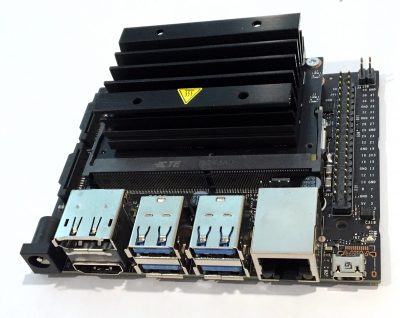
The CUDA version is 9.9x faster than the 6-processor (stochastic) MPI version and 55.5x faster than the serial version! Not bad. In case you want to try this code but your computer does not have an NVIDIA GPU, you can get yourself the $99 Jetson Nano.
Javascript with 2D Canvas
Instead of writing a version that we need to compile first, we could use Javascript to develop an interactive version running in a browser. HTML5 provides a canvas element that allows direct drawing using either a 2D or a 3D context. We can thus write a sample function that picks a random point in the square and visualize it using different color or size depending on whether it is in or out. We also keep track of how many points we sampled and how many were in. We use requestAnimationFrame to have the browser call sample again as soon as possible. Periodically we also update value in span elements to display the current π estimate. This update is done only every 20 samples, on average, to reduce “flickering”.
<!DOCTYPE html> <html> <head> <meta charset="UTF-8"> </head> <body> <canvas width="400" height="400" id="canv">Canvas not supported!</canvas> <div> Using <span id="span_samples">0</span> samples, π is <b><span id="span_pi">0</span></b> <br> <input type="button" value="Start" id="button_start" onclick="start()"></input> <input type="button" value="Reset" id="button_reset" onclick="reset()"></input> </div> <script> // global variables var c = document.getElementById("canv"); var ctx = c.getContext("2d"); var N_in = 0; var N_tot = 0; var running = false; // picks and classifies a single random point function sample() { var x = Math.random(); // pick random number in [0,1) var y = Math.random(); N_tot++; // increment samples counter var r = 5; // default radius var color = "red"; // default color // update size, color, and counter if in circle if (Math.sqrt(x*x+y*y)<=1) { r = 7; color = "green"; N_in++; } // scale and flip y, canvas y=0 is on top x*=c.width; y=(1-y)*c.height; // create gradient for drawing circles var grd = ctx.createRadialGradient(x, y, 0, x, y, 1.3*r); grd.addColorStop(0, color); grd.addColorStop(1, "white"); // draw circle ctx.beginPath(); ctx.arc(x,y,r, 0, 2*Math.PI); ctx.fillStyle = grd; ctx.fill(); // update output on average every 20 steps (to avoid flicker) if (N_tot%Math.floor((Math.random()*20))==0) { var pi = 4*(N_in/N_tot); document.getElementById("span_samples").innerHTML=N_tot; document.getElementById("span_pi").innerHTML=pi.toFixed(5); } // if simulation running, request to be called again ASAP if (running) requestAnimationFrame(sample); } // toggles whether simulation runs, also updates button text function start() { running = !running; document.getElementById("button_start").value = running?"Stop":"Start"; if (running) sample(); // call sample function if running } // resets counts and clears the canvas function reset() { ctx.fillStyle="white"; ctx.fillRect(0,0,c.width,c.height); N_in = 0; N_tot=0; document.getElementById("span_samples").innerHTML=N_tot; document.getElementById("span_pi").innerHTML=0; } </script> </body> </html>
Source: pi-canvas.html but you can also run the code interactively below (press Start to begin):
Javascript with WebGL
The Javascript canvas element also allows us to access the GPU! This is done using a webGL context of the canvas element. The actual code running on the GPU is specified by implementing two shader programs in C++ syntax. In order to draw some shape, we load a list of of vertexes for triangle strips or similar basic elements. The GPU then calls the first shader, called a vertex shader, to transform the vertex positions. This is where we would incorporate any perspective or transformation matrixes if interested. In our code, we simply keep the vertex positions as is. After this shader finishes, we have a list of triangles (fragments) that still need to be painted. The GPU then calls the second shader, called a fragment shader, to set the color of each pixel within the triangle. In our code, we use the pixel position to set its color either red or green, based on whether it is inside the circle or not. Then finally, to actually compute π, we count the number of green pixels. This computation should be done on the GPU for efficiency, but here for simplicity, we just loop over the nodes on the CPU:
var N_in = 0;
var N_tot = gl.drawingBufferWidth*gl.drawingBufferHeight;
var pixels = new Uint8Array(N_tot * 4);
gl.readPixels(0, 0, gl.drawingBufferWidth, gl.drawingBufferHeight, gl.RGBA, gl.UNSIGNED_BYTE, pixels);

 // loop over all pixels and count how many we have with non-zero green component (inside)
for (var u=0;u<N_tot;u++)
  if(pixels[4*u+1]>0) N_in++;   //each pixel is 4 bytes containing RGBA
This code copies the RGBA values from the canvas element into the pixels array.
Since each pixel consists of 4 bytes, we use 4*u+1 to access the u-th green value. The entire code is below:
<!DOCTYPE html> <html> <head> <meta charset="UTF-8"> </head> <body id="body"> <canvas width="400" height="400" id="canv">Canvas not supported!</canvas> <div> Using <span id="span_samples">0</span> pixels, π is <b><span id="span_pi">0</span></b> <br> </div> <script> main(); function main() { // global variables var c = document.getElementById("canv"); const gl = c.getContext('webgl'); if (!gl) { document.getElementById("body").innerHTML="webGL not supported!"; return; } // Vertex shader program const vsSource = ` attribute vec4 aVertexPosition; void main() { // simply copy the vertex position gl_Position = aVertexPosition; } `; // Fragment shader program const fsSource = ` precision mediump float; uniform ivec2 uDims; void main() { float x = gl_FragCoord.x/float(uDims.x); float y = gl_FragCoord.y/float(uDims.y); // paint pixel green(-ish) if inside the circle, red otherwise if (x*x+y*y<=1.0) gl_FragColor = vec4(0,0.8,0,1.0); else gl_FragColor = vec4(1.0,0,0,1.0); } `; // set up the GPU code const shaderProgram = initShaderProgram(gl, vsSource, fsSource); // draw the image drawScene(gl,shaderProgram); // postprocess on the CPU - could be done faster on the GPU // get a buffer containing all pixels var N_in = 0; var N_tot = gl.drawingBufferWidth*gl.drawingBufferHeight; var pixels = new Uint8Array(N_tot * 4); gl.readPixels(0, 0, gl.drawingBufferWidth, gl.drawingBufferHeight, gl.RGBA, gl.UNSIGNED_BYTE, pixels); // loop over all pixels and count how many we have with non-zero green component (inside) for (var u=0;u<N_tot;u++) if(pixels[4*u+1]>0) N_in++; //each pixel is 4 bytes containing RGBA // update screen info document.getElementById("span_samples").innerHTML = N_tot; document.getElementById("span_pi").innerHTML = 4.0*N_in/N_tot; } // uses GPU to color all pixels inside a circle green function drawScene(gl, program) { // Tell WebGL to use our program when drawing gl.useProgram(program); // copy window dimensions to the fragment shader var uDims = gl.getUniformLocation(program, "uDims"); gl.uniform2iv(uDims, [gl.drawingBufferWidth, gl.drawingBufferHeight]); // clear the canvas gl.clearColor(1.0, 1.0, 1.0, 1.0); // Clear to white, fully opaque gl.clearDepth(1.0); // Clear everything gl.enable(gl.DEPTH_TEST); // Enable depth testing gl.depthFunc(gl.LEQUAL); // Near things obscure far things gl.clear(gl.COLOR_BUFFER_BIT | gl.DEPTH_BUFFER_BIT); // copy vertex positions to a buffer, (-1,-1):(1,1) are the extents of a webGL window { const positionBuffer = gl.createBuffer(); gl.bindBuffer(gl.ARRAY_BUFFER, positionBuffer); const positions = [ 1.0, 1.0, -1.0, 1.0, 1.0, -1.0, -1.0, -1.0, ]; gl.bufferData(gl.ARRAY_BUFFER, new Float32Array(positions), gl.STATIC_DRAW); const numComponents = 2; const type = gl.FLOAT; const normalize = false; const stride = 0; const offset = 0; var aVertexPosition = gl.getAttribLocation(program, 'aVertexPosition'); gl.bindBuffer(gl.ARRAY_BUFFER, positionBuffer); gl.vertexAttribPointer(aVertexPosition, numComponents, type, normalize, stride, offset); gl.enableVertexAttribArray(aVertexPosition); } // draw the triangles { const offset = 0; const vertexCount = 4; gl.drawArrays(gl.TRIANGLE_STRIP, offset, vertexCount); } } // this function sets up the GPU code function initShaderProgram(gl, vsSource, fsSource) { const vertexShader = loadShader(gl, gl.VERTEX_SHADER, vsSource); const fragmentShader = loadShader(gl, gl.FRAGMENT_SHADER, fsSource); const shaderProgram = gl.createProgram(); gl.attachShader(shaderProgram, vertexShader); gl.attachShader(shaderProgram, fragmentShader); gl.linkProgram(shaderProgram); if (!gl.getProgramParameter(shaderProgram, gl.LINK_STATUS)) { alert('Unable to initialize the shader program: ' + gl.getProgramInfoLog(shaderProgram)); return null; } return shaderProgram; } // loads shader code from the strings function loadShader(gl, type, source) { const shader = gl.createShader(type); gl.shaderSource(shader, source); gl.compileShader(shader); if (!gl.getShaderParameter(shader, gl.COMPILE_STATUS)) { alert('An error occurred compiling the shaders: ' + gl.getShaderInfoLog(shader)); gl.deleteShader(shader); return null; } return shader; } </script> </body> </html>
Source: pi-webgl.html. The dynamic code output is also shown below:
Arduino Microcontroller
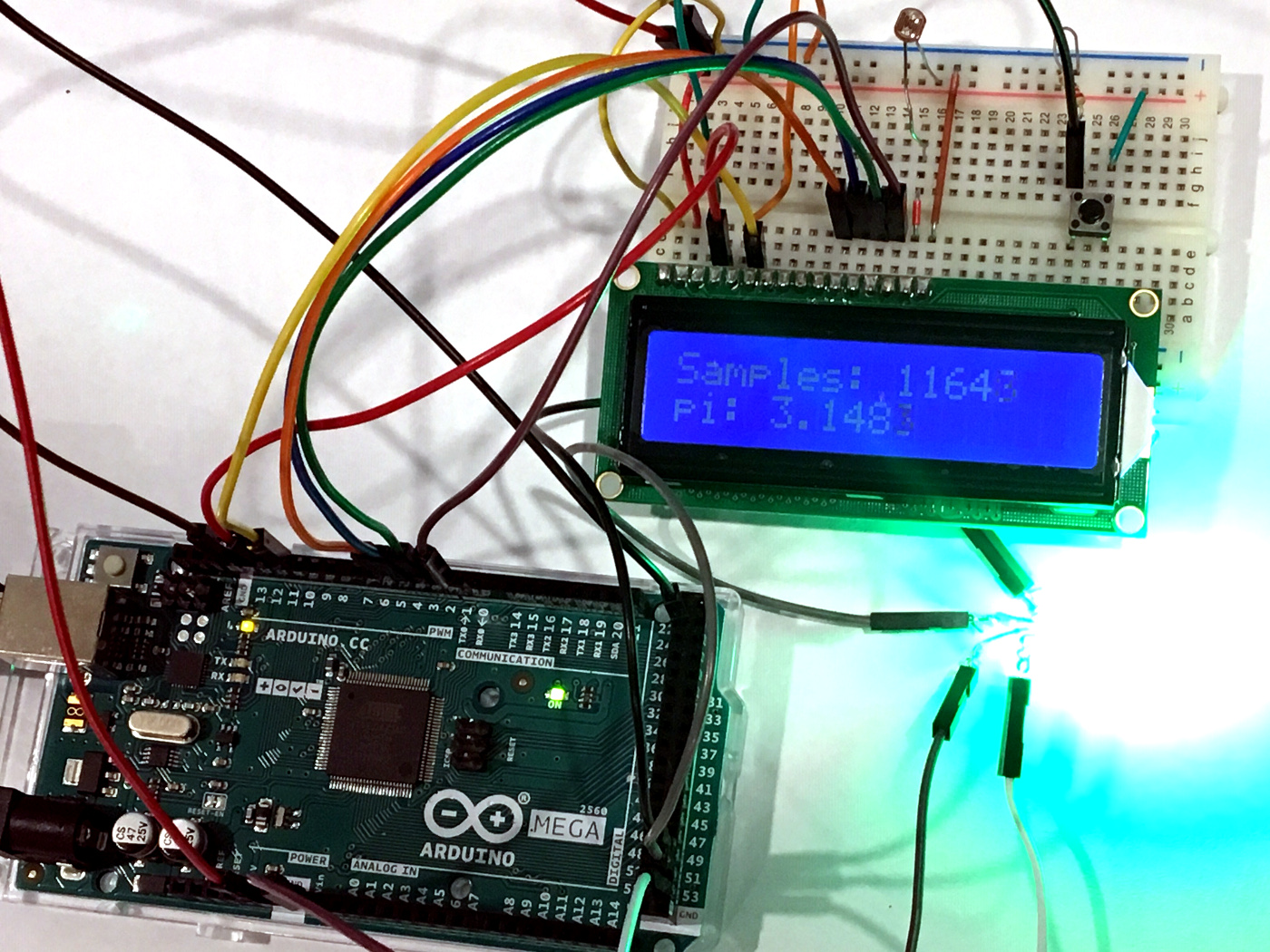
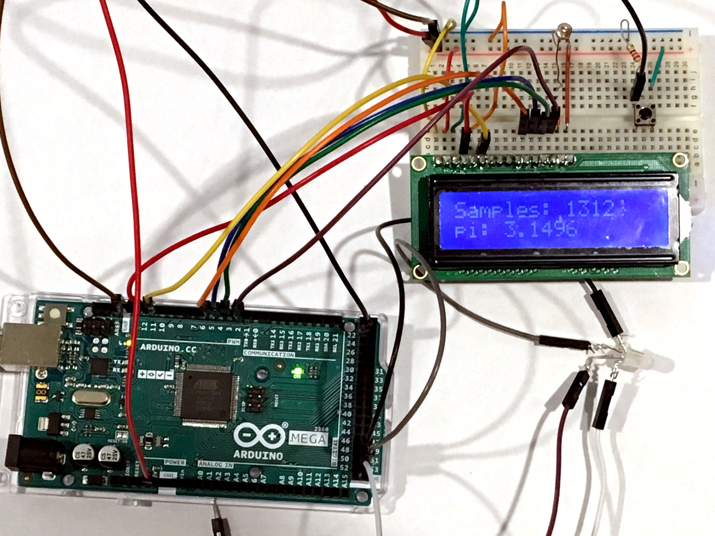
We could also run this simulation on an Arduino Microcontroller. This is basically a small CPU used to drive electrical circuits. Here I used the Arduino Mega board along with the LCD display that comes with the Arduino Starter Kit. I also utilized an RGB LED, a photoresistor, and a switch, plus bunch of wires. The LCD was wired based on the Arduino tutorial, except that I just used some random resistor for the contrast line (V0) and used a photoresistor for the display brightness (LED pin 15). Finally, I also added a button to allow resetting the counters.
So how does all this work? The Arduino code consists of two functions, begin and loop. The first one is executed just once, while the second one is executed repeatedly. The loop function picks a single random number and determines if it is inside the circle or not. If it is, we increment the N_in counter. To make the computation more interesting, we also illuminate an RGB LED green. If the point is outside, we flash the LED red. The way the RGB LED works is that we actually ground the electrode corresponding to the color we want to display. So setting the three pins connected to RGB to (0,0,0) makes the LED shine white. Changing the output to (1,0,0) gives us red color. To simplify this, I added a setLedColor function that works more in the expected way, so that calling it with (1,0,0) gives us red.
The code is artifically slowed down by including delay(50) to wait for 50 ms before picking a new number. This is to make it possible to catch the different colors. I also check for the button press (specifically, button release). This causes the counters to be reset. To provide further feedback, the LED temporarily blinks blue on reset. The check is performed by keeping track of the prior value from the switch read out pin. We perform the reset once the value changes from 1 (pressed) to 0 (released). The output to the LCD is performed using the Arduino LCD library. This library allows us to write character-based messages starting from a specific cursor position.
The Arduino code is given below
#include <LiquidCrystal.h>

// specify pins to use
const int pinButton = 22;
const int pinRed = 53;
const int pinGreen = 51;
const int pinBlue = 49;
const int rs = 12, en = 11, d4 = 5, d5 = 4, d6 = 3, d7 = 2;
LiquidCrystal lcd(rs, en, d4, d5, d6, d7);  // lcd object

void setup() {
  // put your setup code here, to run once:
  Serial.begin(57600);
  pinMode(pinRed,OUTPUT);
  pinMode(pinGreen,OUTPUT);
  pinMode(pinBlue,OUTPUT);
  lcd.begin(16, 2);    // set up LCD dimensions
  setLedColor(0,0,0);  // turn off the LED
  reset();    // initialize counters
}

int button_old = 0;    // the last state of the button
long N_in = 0;
long N_tot = 0;

void loop() {
  // put your main code here, to run repeatedly:
  int button = digitalRead(pinButton);
  if (!button && button_old) reset();
  button_old = button;

  // pick random point
  float x = random(RAND_MAX)/(float)RAND_MAX;
  float y = random(RAND_MAX)/(float)RAND_MAX;
  N_tot++;

  if (x*x+y*y<=1) {      // if inside
    setLedColor(0,1,0);  // green
    N_in++;
  }
  else {
    setLedColor(1,0,0);  // red
  }

  // update pi estimate on the LCD
  lcd.setCursor(9,0);
  lcd.print(N_tot);
  lcd.setCursor(4,1);
  float pi = 4*N_in/(float)N_tot;
  lcd.print(pi,4);

  delay(50);  // wait 50 ms to slow down the LED blinking rate
}

// illuminates the LED to a particular combination of r/g/b
void setLedColor(int r,int g, int b) {
 digitalWrite(pinRed,1-r);
 digitalWrite(pinGreen,1-g);
 digitalWrite(pinBlue,1-b);
}

void reset() {
 lcd.clear();
 lcd.setCursor(0,0);
 lcd.print("Samples:");
 lcd.setCursor(0,1);
 lcd.print("pi:");
 Serial.println("Resetting!");
 setLedColor(0,0,0);
 delay(200);
 setLedColor(0,0,1);
 delay(500);
 setLedColor(0,0,0);
 delay(200);
 N_in = 0;
 N_tot = 0;
}
Source: pi-arduino.ino.
FPGA
Lately I have started playing with FPGAs or Field Programmable Gate Arrays. FPGAs are basically processors that we generate programatically. Instead of having a processor read and execute instructions making up our program, with an FGPA, we basically rewire the processor circuits such that the desired logic is performed. This is pretty neat. FPGAs are typically programmed using hardware description languages, such as VHDL or Verilog. These languages allow us to write the FPGA logic using syntax that is quite similar to higher level languages such C++. Without HDL, we would need to manually implement all the bit-wise operations to perform math operations, which as you can imagine, would be quite tedious! I am still quite new to FPGA programming, but it was not too difficult to write a Verilog version of the grid-based estimator. This code is running serially and the next step should involve taking advantage of FPGA’s parallel capabilities. Future work?
module pi_fpga;
  reg clk;
  integer i,j;
  parameter N = 800;
  real x,y;
  real fi, fj;
  integer N_in;

  initial begin
    clk <= 0;
    i <= -1; j<= 0;
    N_in = 0;
    // $monitor ("T=%0t clk=%0d, i=%0d, j=%0d, x=%0f", $time, clk, i, j,x);
  end

  // create a clock
  always #1 clk = ~clk;

  // code to run on each clock "tick"
  always @ (posedge clk) begin
    i = i + 1;
    if (i>=N) begin
      i<=0;
      j=j+1;
      if (j>=N) begin
        fi = N_in;
        $display("Using %0dx%0d mesh (%0d points), pi = %0f",N,N,N*N,4*fi/(N*N));
        $finish;
      end
    end
    fi = i;
    fj = j;
    x = fi/N;
    y = fj/N;
    if ((x*x+y*y)<=1) N_in <= N_in+1;
  end
endmodule
Source: pi_fpga.v
Similar to the Arduino code, Verilog code can contain multiple initial blocks that execute on program start up. We can also define some always blocks that execute after some condition. There are two such blocks used here. The #1 syntax means “wait for 1 clock cycle”. We use it to implement a hardware clock, with the clk flipping values between 0 and 1. We also define another block that executes on each positive edge of the clk variable – basically whenever the variable goes from 0 to 1. Here the code is fairly standard. We simply increment the i (and optionally j) variable. We then perform the floating point division to obtain \(x\in[0,1]\). I couldn’t figure out a way to cast the int to float in a single operation and hence we use temporary fi and fj floating point variables. The code runs until j goes out of range,at which point we print out the computed value and exit.
We can run a simulation of this FPGA code using iverilog,
$ iverilog pi_fpga.v -o pi_fpga
$ vvp ./pi_fpga
Using 800x800 mesh (640000 points), pi = 3.141519
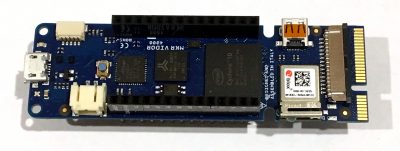
To actually burn it onto an FPGA, we could use program such as Intel’s Quartus. Quartus does not support directly burning onto the Vidor card I have (shown in Figure 10), but there are online tutorials showing you how to do so through the Arduino IDE. Or, you can just get yourself one of the supported boards.
And that’s all. Feel free to leave a comment or suggestions for different technologies to look into.