Interpolation using an arbitrary quadrilateral

In the previous article on the Particle In Cell method (PIC), we introduced the concept of scattering data to the grid. The PIC method relies heavily on the interpolation of data between particles and the grid. First, the scatter operation is used to compute charge density which is then fed to the Poisson solver. The computed electric field, which is stored on grid nodes, is subsequently gathered back onto the particle positions to calculate their acceleration.

Mesh interpolation

The interpolation technique we used in that example is based on linear area weighing. There are other alternatives (see [1] for instance). Some, such as the nearest point method, are less accurate. Others utilize second or higher order scheme to increase accuracy. The linear method described here offers a good compromise between accuracy and the computational overhead. This is the method that is used in all our codes.

This interpolation scheme is summarized below in Figure 1. We want to interpolate some quantity existing at the position denoted by the large red circle to the four grid nodes. To do this, we divide the cell into four sections (or eight in 3D). The fraction to be deposited to each node is simply given by the ratio of the area diagonally opposite from the node to the total cell area, \(w_i=A_i/A\) (in 3D you would use volume ratios). To help you visualize this, in Figure 1, the nodes are shaded with the color corresponding to the area fraction that gets deposited to it.

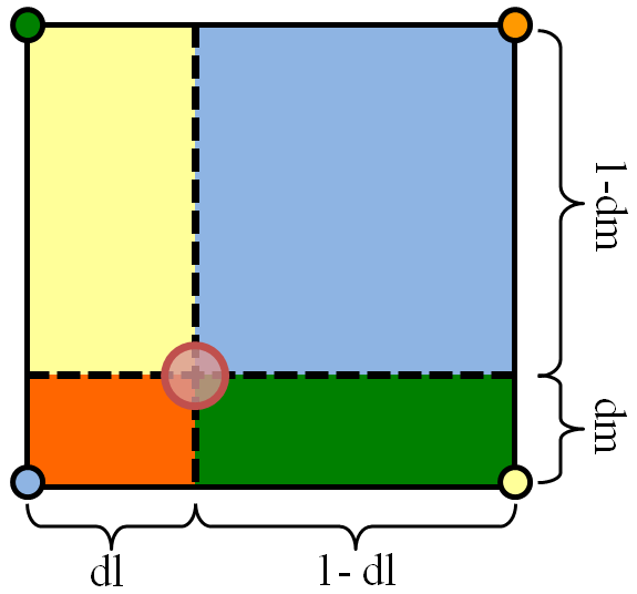
When making this calculation it helps to work in logical (or natural) coordinates. These are coordinates that define the position in the cell as a fraction of the cell distance along the corresponding dimension. In this article we label these coordinates as \(l=[0,1]\) and \(m=[0,1]\). Value of zero corresponds to the left or bottom edge, and value of 1 is the right or top edge. For a Cartesian system such as the one used in the example PIC code we can easily obtain these coordinates as \(i_f=(x-x_0)/\Delta x\) and \(l=i_f-\text{int}(i_f)\) (the “f” subscript was added to indicate that \(i_f\) is a floating point number and not an integer). In logical coordinates the total area is unity, and thus we simply need to multiply the value to be scattered by the corresponding sectional area. The respective lengths are called out in Figure 1. To gather from the grid to the particle we simply multiply the value at each node by the opposite area and add the contributions together, \(n_x = w_1n_1 + w_2n_2 + w_3n_3 + w_4n_4\).

Mapping function for an arbitrary quadrilateral

The above technique works but it has one serious drawback: as written it is useful only for rectangular cells. But often we prefer to use cells that are irregular. Even if we do not use the finite element method, we may want to use method such as finite volume along with cut cells to approximate the surface boundary. Or we may want to use a body-fitted structured mesh. These methods will give us mesh cells that are no longer rectilinear but are arbitrary quadrilaterals. Of course, you could end up with different shapes such as triangles or three dimensional wedges depending on your setup, but here for simplicity we consider only 2D quads. Ref [2] has a good overview of various cell types.

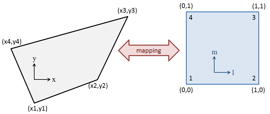
In order to perform the interpolation on an arbitrary quad, we need to obtain a mapping function as shown in Figure 2. Our goal is to come up with a functions such as \((x,y)=f(l,m)\) where \(l=[0,1]\) and \(m=[0,1]\) describes the entire point space enclosed by the quadrilateral. In addition, we want \(f(0,0)=(x_1,y_1)\), \(f(1,0)=(x_2,y_2)\) and so on to correspond to the polygon vertices. This function, yet to be determined, forms a map that allows us to transform the quad from the physical coordinate set to a logical coordinate space. In the logical coordinates, the polygon morphs into a square, regardless of its physical form. Once the logical coordinates are obtained, we perform the scatter and gather operations just as described in the above paragraph.

What remains now is finding the map. To do this, we assume a bilinear mapping function [2] given by
$$x=\alpha_1 + \alpha_2 l + \alpha_3 m + \alpha_4 lm$$
and
$$ y=\beta_1 + \beta_2 l + \beta_3 m + \beta_4 lm$$
We next use these expressions to solve for the four coefficients,
$$ \left[\begin{array}{c}x_1\\x_2\\x_3\\x_4\end{array}\right] = \left[\begin{array}{cccc}1&0&0&0\\1&1&0&0\\1&1&1&1\\1&0&1&0\end{array}\right] \left[\begin{array}{c}\alpha_1\\\alpha_2\\\alpha_3\\\alpha_4\end{array}\right]$$
The coefficients in the matrix come from Figure 2. For instance for node “1” we have (l,m)=(0,0). A similar expression is also written for the betas. We can solve for the coefficients easily by inverting the matrix,
$$ \left[\begin{array}{c}\alpha_1\\\alpha_2\\\alpha_3\\\alpha_4\end{array}\right] = \left[\begin{array}{cccc}1&0&0&0\\-1&1&0&0\\-1&0&0&1\\1&-1&1&-1\end{array}\right] \left[\begin{array}{c}x_1\\x_2\\x_3\\x_4\end{array}\right]$$

Using Matlab syntax, we can write

%create our polygon
px = [-1, 8, 13, -4];
py = [-1, 3, 11, 8];
 
%compute coefficients
A=[1 0 0 0;1 1 0 0;1 1 1 1;1 0 1 0];
AI = inv(A);
a = AI*px';
b = AI*py';

We now have our mapping to go from the logical to the physical world. To obtain the reverse mapping we need to solve
$$\begin{array}{rcl} x&=&\alpha_1 + \alpha_2l +\alpha_3m+\alpha_4 lm \\ y&=&\beta_1 + \beta_2l +\beta_3m+\beta_4 lm\end{array}$$
Note this system is no longer linear, however it can be solved quite easily analytically. You can first obtain
$$l= \left(\dfrac{x-\alpha_1-\alpha_3 m}{\alpha_2+\alpha_4 m}\right)$$
which can then be substituted into the second expression (this is as they say, “an exercise left for the reader”) to obtain
$$(\alpha_4\beta_3 – \alpha_3\beta_4)m^2 + (\alpha_4\beta_1-\alpha_1\beta_4+\alpha_2\beta_3 -\alpha_3\beta_2 + x\beta_4 – y\alpha_4)m + (\alpha_2\beta_1 – \alpha_1\beta_2 + x\beta_2 – y\alpha_2)=0$$
This is simply a quadratic equation with the three coefficients given by the terms in the parentheses and with the physical solution \(m = (-b + \sqrt{b^2-4ac})/2a\). The Matlab/Octave function below does this calculation and converts the supplied physical coordinates to logical ones using the also-supplied coefficients.

% converts physical (x,y) to logical (l,m)
function [l, m] = XtoL(x,y,a,b)
    %quadratic equation coeffs, aa*mm^2+bb*m+cc=0
    aa = a(4)*b(3) - a(3)*b(4);
    bb = a(4)*b(1) -a(1)*b(4) + a(2)*b(3) - a(3)*b(2) + x*b(4) - y*a(4);
    cc = a(2)*b(1) -a(1)*b(2) + x*b(2) - y*a(2);
 
    %compute m = (-b+sqrt(b^2-4ac))/(2a)
    det = sqrt(bb*bb - 4*aa*cc);
    m = (-bb+det)/(2*aa);
 
    %compute l
    l = (x-a(1)-a(3)*m)/(a(2)+a(4)*m);
end

Example 1: Picking random points in a quadrilateral

Now we have everything we need to have some fun. The first example shows how to pick random points that are located within a prescribed quad. Any point located within the polygon will have natural coordinates in the 0 to 1 range. Hence we just need to pick two random natural coordinates and convert them with the mapping function. The code is given below. The real part is the part in the loop – the second half is simply a code to generate the plot. You will get a plot similar to the one in Figure 3, however the actual point locations will vary. Notice that all points are located within the polygon bounds.

%plots random points inside the polygon
function []=plot_points_in_poly(px,py,a,b)
 
    %pick random logical coordinate and convert to physical
    for i=1:100
	l=rand();
	m=rand();
	x(i) = a(1) + a(2)*l + a(3)*m + a(4)*l*m;
	y(i) = b(1) + b(2)*l + b(3)*m + b(4)*l*m;	
    end
 
    %plot
    figure(1);
    hold off;
    plot([px px(1)],[py py(1)]);
    hold on;
    plot (x,y,'x');
end

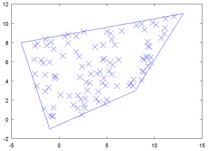
Figure 3. Plot of 100 random points all located inside the polygon.

Example 2: Determining if a point lies inside or outside the quadrilateral

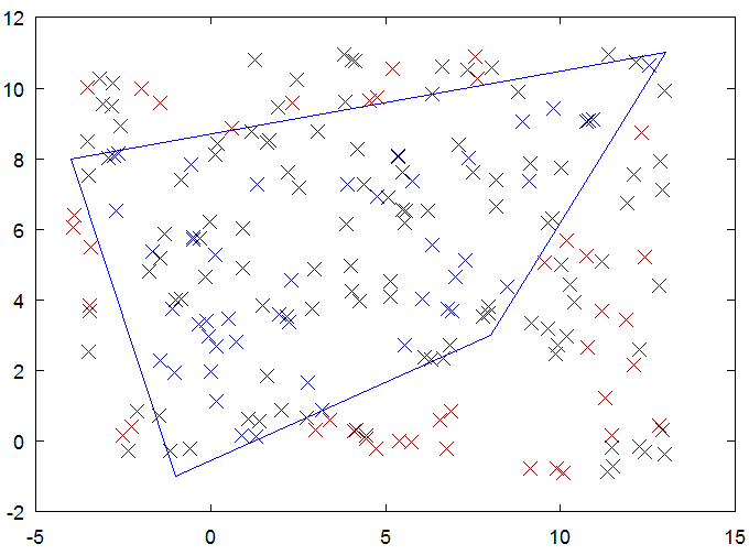
The first example showed how to go from the logical to the physical coordinates. The second example is the opposite. In this example we pick 200 points randomly distributed in the polygon bounding box and determine if they are inside or outside the polygon. To accomplish this, we use the fact that a point inside the polygon will have both natural coordinates in the 0 to 1 range. Although here we simply flag the node location, a variant of this technique could be used in an unstructured code to search for the cell containing a particle. A coordinate \(m>1\) indicates that the next searched cell should be the one sharing the \(m=1\) edge (whatever this means physically depends on the mapping). This is much faster than looping through the cells one by one. When you run the code below, you will get a plot similar to the one in Figure 4

%picks random points and colors them based on internal or external
function []=plot_internal_and_external_points(px,py,a,b)
 
    %bounding box
    x0 = min(px);
    lx = max(px)-min(px);
    y0 = min(py);
    ly = max(py)-min(py);
 
    %convert random physical coordinates to logical
    for i=1:200
 
  	%pick a random point in the bounding box
	x(i) = x0+rand()*lx;
	y(i) = y0+rand()*ly;
 
	%calculate logical coordinates
	[l,m] = XtoL(x(i),y(i),a,b);		
 
	%is the point outside the quad?
	if (m<0 || m>1 || l<0 || l>1)
		type(i)=1;
	else
		type(i)=0;
	end
    end
 
    %plot
    figure(2);
    hold off;
    plot([px px(1)],[py py(1)]);
    hold on;
    scatter(x,y,4,type,'x');
end

Example 3: Scattering data to polygon nodes

Next we consider something of actual use to the PIC method: the scatter operation. Here we pick 100 random points inside the polygon and scatter the value of “1” for each point. This in essence counts the number of points in the polygon. Given a large number of samples and a good random number generator, we should get the value of 25 at each node. In the code below we scale this data such that the expected value on each node is 10 (this was done for visualization purposes). When I ran the code below I got:
9.8026 9.6121 9.8507 10.7346
These values add up to 40 as expected. Figure 5 shows this data graphically with the size of the circle corresponding to the node value. If the density was not uniform, we would see the circles have varying sizes.

%scatters counts to the four grid nodes
function []=scatter_data(px,py,a,b)
 
    %init
    c = [0 0 0 0];
 
    %pick random logical coordinate and convert to physical
    for i=1:100
 
 	%random point inside the quad
	l=rand();
	m=rand();
 
	%deposit counts, note here l,m=[0:1]. In a real 2d mesh
	%the index we would first need to subtract the integral
	%cell index to get the cell-local distance, dl = l - (int)l;
	dl = l;
	dm = m;
 
	c(1) += (1-dl)*(1-dm);
	c(2) += dl *(1-dm);
	c(3) += dl * dm;
	c(4) += (1-dl)*dm;
    end
 
    %scale data, uniform distribution = 10
    c = 40*(c/i);
 
    %output
    disp(c);
 
    %plot
    figure(3);
    hold off;
    plot([px px(1)],[py py(1)]);
    hold on;
    scatter(px,py,c,[1 0 0], 'o');
end

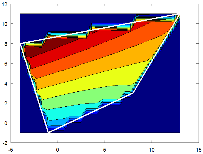
Example 4: Gathering data from polygon nodes onto a particle

And finally, here is the opposite of the previous example. Here we interpolate data from the grid nodes onto the particle position. This is analogous to gathering electric field components prior to evaluating acceleration. In this example we set the values [1,2,3,4] onto the polygon vertices. To better illustrate this interpolation, we construct a 30×15 uniform grid and interpolate the polygon values onto the grid points. We only do this for points located inside the polygon. The 2D grid allows us to visualize the results as a contour flood. The example starts by constructing the grid. It then loops through the grid nodes and performs the calculation using each grid node position. The output is shown in Figure 6.

 
%interpolates data from the polygon vertices onto a grid
function []=gather_data(px,py,a,b)
 
    %bounding box
    x0 = min(px);
    lx = max(px)-min(px);
    y0 = min(py);
    ly = max(py)-min(py);
 
    %set spacing such that we have 30x30 grid (i.e. 29 cells)
    ni = 30;
    nj = 15;
 
    dx = lx/(ni-1);
    dy = ly/(nj-1);
 
    %node positions (for plotting)
    for i=1:ni
 	x(i) = x0 + (i-1)*dx;
    end
    for j=1:nj
 	y(j) = y0 + (j-1)*dy;
    end
 
    %node values
    c = [1 2 3 4];
 
    val=zeros(nj,ni);
 
    for i=1:ni
	for j=1:nj
             %convert to logical coordinates
	     [l m] = XtoL(x(i),y(j),a,b);	
 
	     %evaluate only if we are inside
	     if (l>0 && l<=1 && m>=0 && m<=1)
 
                 %again, if we had multiple cells, we would set dl = l - (int)l
	         dl = l;
	         dm = m;
 
	         val(j,i) = (1-dl)*(1-dm)*c(1) + ...
		    	        dl*(1-dm)*c(2) + ...
			        dl*dm*c(3) +...
			    (1-dl)*dm*c(4);		
             end
        end
    end
 
    %plot
    figure(4);
    hold off;
    contourf(x,y,val);
    hold on;
    plot([px px(1)],[py py(1)],'w','LineWidth',4);
end

Complete Source Code

You can get the complete source code here: interpolate2d.m.

As an aside, this code was tested using Octave 3.2.4, and not Matlab, since I do not have a copy of the latter. Octave is a free open source Matlab emulator than can be downloaded from octave.org or as a Cygwin package. The Cygwin version is newer (version 3.6.2 as of writing) but since it requires few additional steps such as (1) installing Cygwin and (2) installing XWin I used the older (and quite buggy) pre-built Windows version from the Octave site.

References

[1] Birdsall, C. K., and Langdon, A.B., “Plasma Physics Via Computer Simulations“, Institute of Physics Publishing, 2000

[2] Hughes, T. J. R., “The Finite Element Method“, Dover Publications, 2000