The Electrostatic Particle In Cell (ES-PIC) Method

Particle-In-Cell (PIC) is a technique commonly used to simulate motion of charged particles, or plasma. Here I show you the basics of the method, as applicable to studies of phenomena such as solar wind propagation, or analysis of electric thruster plumes. These discharges are characterized by low plasma densities. At low density, plasma behaves more like a collection of discrete particles, than a single continuous fluid. High-density plasmas are simulated using the extension of computational fluid dynamics into electromagnetics, magnetohydrodynamics.
Modeling of plasmas is complicated by the presence of external and self-induced electromagnetic fields, inter-particle interactions, presence of solid objects, and the different characteristic time scales at which ions and electrons propagate. In order to speed up the calculation, simplifying assumptions are generally taken to match the problem at hand. Here, we are assuming that the current generated by the plasma medium is low enough so that the self-induced magnetic field can be ignored. This is a valid assumption for the class of problems we are dealing with here. As such, the set of underlying Maxwell’s equations is reduced and we obtain an Electro-Static PIC code. In addition, we assume that electrons follow the Boltzmann relationship. The simulation then consists of only the heavy particles, ions and neutrals. This simplification has a tremendous impact on the computational speed, since the time integration can be performed on the much larger ion time scale. Finally, we assume that gas densities are sufficiently low so that particle collisions are negligible.
So what is plasma? It is a collection of charged particles (ions and electrons) as well as non-ionized atoms that is globally charge neutral. In other word, assume that you could grab a chunk of plasma. As long as the radius of this volume is larger than a certain characteristic length (called the Debye lenght), the collection will contain approximately equal amount of positive (from ions) and negative (from electrons and negative ions) charge. The ratio of ionized particles to neutral atoms is the ionization fraction. In
electric thrusters, about 90% of the working gas is ionized.
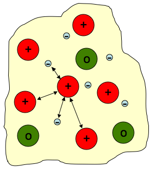
Figure 1. Representation of plasma as a collection of ions (+), electrons (-) and neutral atoms (o). Charged particles interact with each other through self-induced electric fields.
Charged particles interact with each other by attracting particles of opposite charge and repelling those with the same charge. This is the Coulomb force and is given by: \(\vec{F}=\dfrac{1}{4\pi\epsilon_0}\dfrac{q_1q_2}{r^2}\vec{r}_{12}\). Conceptually, we could simulate plasma by taking a collection of particles representing the real physical ions and electrons and directly computing this force. However, plasma simulations generally require at least 1 million particles in order to reduce numerical errors. Since Coulomb force leads to an n2 problem, computation of a single time step would require at least 1 trillion operations. Quite a daunting task, especially considering that a typical simulation requires several thousand of such steps!
Introducing the Particle-In-Cell (PIC) method. This method also uses computational particles (called macro-particles) to represent the real ions, electrons and neutrals. However, instead of computing the Coulomb force directly, we obtain the force acting on the particles from the electric field. Force acting on the particles is given by the Lorentz force, \(\vec{F}=q\left(\vec{E}+\vec{v}\times\vec{B}\right)\), which is a size-n problem. Here q is the particle charge, E is the electric field, and v and B are the particle velocity and magnetic field, respectively. In this example we will assume that plasma is not subjected to any magnetic field (self-induced or applied) and thus the second term in the Lorentz force equation can be ignored. As was eluded to previously, it is not computationally feasible to simulate every physical ion, electron or neutral. As such, each computational particle represents a large number (several tens of million in thruster simulations) of real particles. The ratio of real particles per macro-particle is called the specific weight, sp_wt.
Fundamental Equations
Motion of each macroparticle is governed by Newton’s Second Law,
$$\begin{align}
\frac{d\vec{x}}{dt}&=\vec{v}\\
\frac{d\vec{v}}{dt}&=\frac{q}{m}\vec{E}
\end{align}$$
Here \(q\) is the particle charge and \(m\) is the particle mass. Electric field is computed from \(\vec{E}=-\nabla\phi\), where \(\phi\) is the electric potential. It is given by \(\nabla^2\phi = -\dfrac{\rho}{\epsilon_0}\), the Poisson equation. Here \(\rho\) is the charge density and \(\epsilon_0\) is the permittivity of free space. In terms of ion and electron number densities, charge density is written as \(\rho=e(Z_in_i-n_e)\). The subscripts i and e denote ions and electrons, respectively, and \(Z_i\) is the average ion charge number.
Due to their tiny mass, electrons move at very high velocities (on the order of 5×10⁵ m/s in the types of plasmas considered by MpNL). Resolving electron motion without introducing numerical errors requires the use of extremely small computation time steps (around 10-12 s). With such a small time step, it is not feasible to study any large-scale problems. For instance, it takes couple tens of µs for an ion beam to propagate several thruster lengths from the spacecraft. At the electron time scale, such a simulation would require 10 million time steps. In addition, from the frame of reference of the ions, electrons move instantaneously. Hence it makes sense to simplify the analysis by considering electrons as a fluid. The electron density is then given by the Boltzmann relationship,
$$n_e=n_0\exp\left(\frac{\phi-\phi_0}{kT_e}\right)$$
The Algorithm
The Particle In Cell method consists of an initial setup, the main loop, and a final clean up / results output. All computation happens in the loop. The loop consists of the following steps:
- Compute Charge Density: particle positions are scattered to the grid
- Compute Electric Potential: performed by solving the Poisson equation
- Compute Electric Field: from the gradient of potential
- Move Particles: update velocity and position from Newton’s second law.
- Generate Particles: sample sources to add new particles
- Output: optional, save information on the state of simulation
- Repeat: loop iterates until maximum number of time steps is achieved or until simulation reaches steady state
Compute Charge Density
Charge density is a scalar variable spatially varying in space. It indicates the number of charge units per unit volume. We compute it by distributing charge of all particles onto the nodes of computational cells, and then dividing by the corresponding node volume.
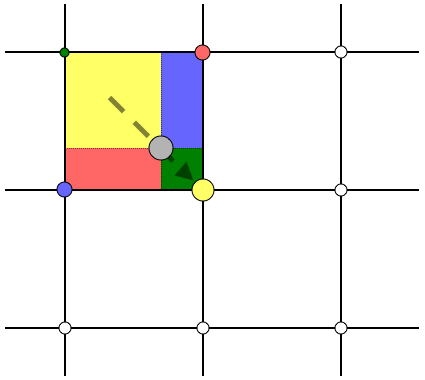
Figure 2. Schematic of the scatter operation. Charge of the particle (in gray) is distributed among the surrounding nodes. Charge contributed to each node is based on the proximity of the particle to that node.
The 1st order (linear) scatter operation is schematically shown in Figure 2. This figure shows a snippet of the computational mesh, and the simulation particle, shown in gray. Charge of the particle is distributed among the nodes of the cell the particle is in. Hence then name for this method, particle in cell. Please note that the total charge carried by each macro-particle is sp_wt*q. The yellow node receives the largest fraction, due to the particle’s close proximity to this node. The smallest amount is contributed to the green node. The weight factors are given by the four area fractions,
$$\begin{align}
w_1 &= (1-h_x)(1-h_y)\\
w_2 &= (h_x)(1-h_y)\\
w_3 &= (1-h_x)(h_y)\\
w_4 &= (h_x)(h_y)\\
\end{align}$$
where 1, 2, 3 and 4 correspond to the blue, yellow, green and pink nodes, respectively. hx is the fractional distance of the particle from the cell origin in the x direction. Node volumes equal the cell volumes, ΔxΔy. Exceptions exist along domain boundaries, since here only a half (or quarter for corners) of cells is contributing. More complicated boundary conditions require additional treatment. For instance, periodic boundaries require summation of nodes on the plus (+) and the negative (-) side of the domain. This interpolation technique can also be used to scatter data with non-rectangular cells by mapping the physical coordinates to a regular logical domain.
Compute Electric Potential
Next, the electric potential is calculated by calling an elliptic equation solver. The Poisson equation can be discretized as
$$ \frac{\phi_{i-1,j}-2\phi_{i,j}+\phi_{i+1,j}}{\Delta^2x}+\frac{\phi_{i,j-1}-2\phi_{i,j}+\phi_{i,j+1}}{\Delta^2y}=-\frac{e}{\epsilon_0}\left[n_i-n_0\exp\left(\frac{\phi-\phi_0}{kT_e}\right)\right]$$
where we used the finite difference with central differencing. This method is modified along mesh boundaries. An elliptic equation describes a boundary value problem and as such boundary conditions must be prescribed along all boundaries. Two types of boundaries exist: Dirichlet and Neumann. The first, Dirichlet, specifies the value of potential. The second boundary specifies the value of the derivative, or electric field. Plasma problems will typically contain a combination of both boundary types. For instance, Figure 3 shows the boundary conditions for the flow of solar wind around a charged plate problem simulated by the sample MATLAB PIC code.
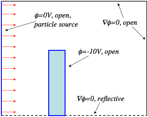
Figure 3. Mix of boundary conditions in the sample PIC code.
Compute Electric Field
Electric field is computed by differencing electric potential, \(E_{x,i}=-\dfrac{\phi_{i+1,j}-\phi_{i-1,j}}{2\Delta x}\) or along boundaries \(E_{x,i}=-\dfrac{\phi_{i+1,j}-\phi_{i,j}}{\Delta x}\). Only the x direction derivative is shown here, and the one sided boundary equation is applicable to the x- face. The remaining derivatives are obtain in an analogous fashion.
Move Particles
We next integrate particle motion through a time step Δt. The Leapfrog method is commonly used in PIC codes. It is fast and numerically stable. First, we integrate velocity through the time step. Next, position is updated. The name comes from the fact that times at which velocity and positions are known are offset from each other by half a time step. As such, the two quantities leap over each other. This idea is sketched in Figure 4.
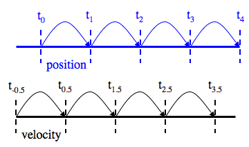
Figure 4. The Leap-Frog method.
Numerically, the particle push is given by
$$\begin{align}
\vec{v}^{k+0.5}&=\vec{v}^{k-0.5}+\frac{q}{m}\vec{E}\Delta t\\
\vec{x}^{k+1}&=\vec{x}^{k}+\vec{v}^{k+0.5}\Delta t
\end{align}$$
The electric field at the position of each particle is computed by a gather operation, which is inversely analogous to the process used to compute charge density.
After particles are moved to new positions, it is necessary to verify that all particles are still in the computational domain. Two boundary interactions are possible. The particles can either exit the domain, or can collide with solid objects. Computational boundaries are either open (or absorbing, allowing particles to leave), reflective (elastically returning particles into the domain) or periodic
(particles are transported to the opposite side of the domain). The reflective boundary is used to identify planes of symmetry. Details of particle-surface interaction, which can result in erosion of native material, is not considered here.
Generate Particles
New particles are generated by sampling sources. Sources include spacecraft thrusters or solar wind. This step is problem specific.
In some cases, all particles will be loaded initially, and the simulation will only computes their final distribution state. Typically we are interested in sampling the Maxwellian distribution. As given in Birdsall, this distribution can be approximated as:
$$f_M=\sqrt{\frac{M}{12}}\left[\sum_{i=1}^{M}R_i-\frac{M}{2}\right]$$
where M is some number and Ri is an i-th random number in range [0:1). The value chosen for M controls the accuracy of this method. Birdsall used 12 to prevent entries larger than 6 times the thermal velocity. In the sample MATLAB code, we use M=3.
Finally, since the Leap-Frog method requires velocity and position to be offset from each other, it is necessary to update the velocity of sampled particles by -Δt. This step is frequently omitted. The size of the numerical error introduced by this omission will depend on several factors: the strength of the electric field near the source and size of the time step. This step is also omitted in the sample code, for clarity as it would require duplication of the velocity update code.
Output
Output from PIC codes includes the spatial distribution of plasma parameters such as potential, charge density, electron temperature, as well as particle data such as velocities and current densities. In addition, time-dependant output of global aggregate diagnostic data, such as total kinetic and potential energy of the simulation, is helpful in diagnosing code performance.
Repeat
The loop repeats until some condition is satisfied. Simulations with continuous sources are run until a steady state is achieved. The steady state is characterized by the net number of particles in the simulation domain remaining constant between time steps. In other words, the number of new particles generated by sources is balanced by the number of particles leaving the domain through the boundaries.
Further Reading
- Birdsall, C.K. and Langdon, A.B.,Plasma Physics via computer simulation, 1985
- Chen, F.F., Introduction to plasma physics and controlled fuison, 1984
- Lieberman, M.A., and Lichtenberg, A.J., Principles of plasma discharges and material processing, 2005
That’s it. Next see the simple Particle In Cell code in Matlab post for implementation and two-stream instability for more. You may also be interested in a PIC code in cylindrical coordinates.
Feel free to leave a comment if you have any questions.
Hi, I am a PhD student studying plasma physics and using the PIC method. I am having trouble to calculate the v x B term of the Lorentz equation. Could you please give me information on how to solve the equation using the leapfrog method?
Best Regards,
Etienne.
Hi Etienne,
Actually the next article I will write for the blog will be exactly on this topic. It should be online by the end of the week. Is that ok? But to get you started, you want to use the method of Boris, or some form of it. It basically consists of half acceleration, full rotation, and then another half acceleration. Do you happen to have a copy of Birdsall’s Plasma Physics via Computer Simulations? (If not you should get it, it’s the bible of PIC). Check on page 61 (Implementation of the vxB rotation).
Great site here.
Since I have to understand the Boris integrator for my master thesis, I have written a short document about it. Maybe it helps you, Etienne, so you don’t necessarily have to get the book: You can obtain it at http://n.ethz.ch/~toggweim/boris.pdf.
Equation (10) is still in implicit form, but you can solve the 3×3 system easily (for example by hand with the Cramer rule). The method is then fully explicit.
By the way, my master thesis is about an integrator for PIC code that uses a global, adaptive time step to increase efficiency. If you have heard of previous attempts or have good ideas please let me know. The main idea is to evaluate the space charge field less often than external fields (in a multiple time stepping fashion), since the space charge solver is the slowest part in the integration procedure.
Regards,
Matthias
Thanks for sharing your write up, Matthias. By the way, I am still working on the integrator article, I am hoping to get it done this week. The problem is finding a good example to illustrate the difficulty with standard integration.
I am really looking forward to see that article!
Interestingly Boris can be derived under a different viewpoint than mentioned in the book, namely as composition of a first order method with its adjoint method, where the first order method is obtained with a splitting approach. (Have almost written this down if you’re interested in more details)
What do you mean with “standard” integration? Have you tried just a single particle in a constant magnetic field that flies a circle? Otherwise, a 2D thing where the magnetic field is a restoring force linear in one coordinate (B(x)=-k*x) should be enough to demonstrate the errors in motion.
Hi Etienne, I’m PhD student too. I use the PIC method to study the electron beam acceleration by a standing electromagnetic field in static inhomogeneous magnetic field based in cyclotron autoresonance phenomenon. I use the Boris method to solve the motion equation. It work very well. If you have any problem still please let me know.
Eduardo.
Hi,
I am a PIC developer. Did you have tried to follow Section 4-4 of Birdsall & Longdon?
The link “MATLAB PIC code” is dead. Can you make the respective content available again?
Will do (and will resume posting articles shortly as well). It’s total crunch time here trying to finish a paper for the upcoming International Electric Propulsion Conference and also submit some proposals…
Great hammer of Thor, that is powerfully helpful!
admin note: this got marked as spam but the comment was too funny not to let it go through…
If I want to simulate different populations of plasmas with different densities, do I just allocate a certain ratio of particles to that population to represent the density? Or are there other ways how I can do this?
Hi Etienne, yes, you can easily include multiple particle species with the PIC method. Most of my codes use a fixed specific weight (number of real particle represented by each macroparticle) for each species. This number should be corresponding to the species density. For good statistics, you want to have at least 10-20 particles per cell. This means that you will need to reduce the specific weight for lower density species. Conversely, you will want to increase it for high density species so that you don’t slow down your simulation with too many particles.
Do you have an upgrading of the Matlab-program in 3D? I have to determine the potential damping of a charge by Debye length. In my Problem, I have a sphere with radius r=Debyelength.
Thank you very much.
Hi Sam,
I have a general 3D plasma simulation code but that one is not publicly available. However, it seems your problem would be solved even easier in 1D, by switching to the spherical coordinate system, no?
Hi,I am phd student in laser plasma interaction and I am looking for to find a 2D-Electromagnetic open source PIC code. Please let me know if you have any recommandation in this regards.
All the best
Hi Elnaz, I have never used it but I believe that OOPic can be used for EM simulations, see http://ptsg.eecs.berkeley.edu/ for more details.
Hi Lubos, Do you know any article where it is discussed in details the issue of determining the minimum number of particles per cell and the related accuracy issues. I understand this number will vary depending on the nature of the problem and the plasma conditions, and at times we may need to use hundreds of particles per cell. Can you give some insight on this issue. Thanks in advance.
Hi Chaudhury, I don’t know of any paper off the top of my head but the number I have heard is 20 particles per cell. But as always, this will depend on your setup. The particle count gives you two things. First, it decreases the smallest charge unit that can be scattered to the grid. This is especially important if you have a high variation in density, such as when you are doing plume analysis. A higher number will then reduce the gradients along the beam edge. Secondly, the higher number allows you to better resolve the velocity distribution function. This is especially true if you use fixed particle weight (as is for instance the case in my old 3D code Draco). Since we typically load Maxwellian distribution, the larger number gives you a better hope of capturing the high energy electrons that are responsible for much ionization in discharges. But in a sense these particles-per-cell numbers are somewhat meaningless. We typically study electric propulsion plumes, and it is not uncommon to have few thousand particles per cell in the high density region and only a few in the wake. Mesh stretching and variable particle weights can help but these are sometimes tricky to implement correctly.
Hi Lubos,
I was wondering if the PIC code can be used for description of arcing between electrodes. The arcing may be caused by lightning.
Yes in theory, however, how practical it will be will strongly depend on the arc density. PIC is typically more suitable for rarefied flows. This is because as the density increases, the computational requirements for the PIC method grow drastically. Also, the main advantage of kinetic methods is that they don’t assume the Maxwellian distribution function. Rarefied flows may deviate from the Maxwellian since there may not be enough particle interactions to thermalize the flow. In dense flows, thermalization is typically quite rapid, so you may be better off using a fluid based approach, such as magnetohydrodynamics.
Thanh you for the great blog! I have a question, how can we introduce the pressure in the code?
This is handled by adding collisions, either with MCC or DSMC methods. With DSMC, you simply add more particles in one area than other and since there is more of them, they will also collide more frequently. The random scattering will then result in the particles diffusing out until you reach an equilibrium situation.
Dear Lubos,
Thank you for the fun PIC code. Quick question. Maybe I misunderstood the problem you are solving, but should not the density be zero inside the rectangular object.
Thank you,
Ales
Hi Ales, it should be and is, but it may not look like it because of the coarse mesh.
Hi
I am working on a 1D electromagnetic PIC code. I have a problem in solving Maxwell’s equations.
In fact when there is a a spatially uniform current density, based on “dE/dt=-4Pi*J”, It give rise to a spatially uniform electric field which oscillates with time, exp(wp*t). This is an undesirable answer.
Would you please tell me how can I resolve this problem.
Thank you
Davood
please help me..how to installation of pic simulation.i want to do my project work in master
Hi there,
Sorry if this is not the relevant place to put it but I have a question about self-force in PIC codes. I have read that if you use the same weighting scheme for density and field interpolation, particles will not exhibit a self force. Is this true even for just one particle in the domain? I am running the two-stream instability on my own PIC code that I have developed and it is very sensitive to the neutralising background ion density. A slight charge imbalance leads to non-physical behaviour. I have used another pic code in the past and it didn’t even need the neutralising ion background nevermind being this sensitive to it. So i am wondering if it is some sort of self-force going on somehow.
Thanks,
Sam
Hi Sam,
What interpolation scheme are you using? Also, you may be interested in signing up for my ES-PIC course. We will be talking about 1D electron simulations next week. You missed the first lecture, but the lecture recordings are available for download.
Hi Lubos,
I am using the first-order weighting scheme as described in Birdsall, calculating the offset and using this to determine how much charge is deposited on the neighbouring grid points. I am using the finite-difference method to solve Poisson’s equation rather than using FFT’s so my boundary conditions may be an issue
I would think that a particle will always exhibit a self force unless it is in the middle of two grid points. A particle that is not in the middle will deposit more of its charge to the grid point closest to it and less to the other grid point. It will then feel a stronger force from the grid point it is closest to so will be pushed away from the gridpoint it was closest too.
Hi,thank you for the PIC code,and I rewrited it with c++.We all know thar electromagnetic wave will decay when propagating in plasma.How to simulate this phenomenon with PIC? Thanks.
That requires an EM-PIC code. I am planning on posting an example shortly.
Thanks for your reply.I am looking forward to your example.
Hello ChenMinQi
I am also working on writing the PIC code in c++ , can you help me with the same ?
Hi Lubos
I am working on simulation of electron and ion sheet by particle In-cell. I see a problem when I imply boundary condition (the boundary is in the bulk plasma) the density of specious arise suddenly on the boundary. Do you know about it?
Thanks.
Hi Mehdi, I am not sure I fully follow. What are your boundary conditions and problem set up? Perhaps you could email me a short summary?
Hi Lubos
In your code where you generate particles, you use the following statements for the particles velocities:
part_v(np+1:np+np_insert,1) = v_drift+(-1.5+rand(np_insert,1) + …)*vth;
part_v(np+1:np+np_insert,2) = 0.5*(-1.5+rand(np_insert,1)+…)*vth;
How are the Right hand side equations defined? Where do you get them from ?
That’s supposed to correspond to sampling from the Maxwellian distribution, using a simple model from Birdsall, $$v_M=v_{th}\left(\sum_{i=1}^M R_i-\frac{M}{2}\right)\left(\frac{M}{12}\right)^{-\frac{1}{2}}$$
For 3 random numbers, this simplifies to \(v_M=\sqrt{2}v_{th}\left(R_1+R_2+R_3-1.5\right)\). The \(\sqrt{2}\) comes from a slight difference between how Birdsall defined the distribution function and how Maxwellian is typically defined, basically, his \(v_{th}=\sqrt{1/2}v_{th}|_M\). It should probably be added to the code above.
So are you saying I should change the above statements as follows:
part_v(np+1:np+np_insert,1) = v_drift+(-1.5+rand(np_insert,1) + …)*sqrt(2)*vth;
part_v(np+1:np+np_insert,2) = 0.5*(-1.5+rand(np_insert,1)+…)*sqrt(2)*vth;
Should I erase out the v_drift in the first equation, and the 0.5 factor in the second?
Hi Lubos,
Just a very quick question on your PIC code. What is the general rule you follow to apply the size of your cell? Like can I have another value apart from dcell = Debye? What are my limitations?
The dcell=debye is needed if solving Poisson’s equation. Otherwise if you assume quasineutrality, you can get away with larger cells. Still, the cell is the smallest size across which you can resolve changes in various properties. The cell size then may be a function of what is it that you are trying to resolve. If you have a beam that is 5 cm across, then a 2 cm cell size will give you only two or three nodes across the beam. Not quite enough to resolve details. But if you are modeling the space environment around a GEO satellite, then 20 cm cell may be quite sufficient.
Hi Lubos,
Just another quick question. For this PIC code if I wanted to have reflective conditions, rather than absorbing conditions on the box, and all other regions I assumed I could modify the if loop as follows:
if (part_x(p,1)=Lx || part_x(p,2)>=Ly || in_box)
part_x(p,:) = -part_x(np,:);
part_v(p,:) = -part_v(np,:);
end
But when I run the code I seem to get the following error where:
“Subscript indices must either be real positive integers or logicals.
Error in flow_around_plate (line 158)
chg(i,j) = chg(i,j) + (1-hx)*(1-hy);”
I’m not sure why it is affecting this part of the code?
I would appreciate if you could clarify.
The reflection of position is probably not right. You need to take into account the domain boundary, which is not necessarily going to be at “0”.
hy i need to install the PIC code, can you help me?
Hello, I have a question on finding the electric field at the boundaries. You say that E_{x,i}=-\dfrac{\phi_{i+1,j}-\phi_{i,j}}{\Delta x}. Say I have a mesh grid with 2 dimensions. Then the ith point is each mesh point in the y direction, and the jth point is each mesh point in the x direction. So [1,2] would be one down, two across (I’ve set my origin as the top left of this is grid).
The equation for E_{x,i} then causes me a problem. As along the boundary, i+1 and j+1 do not exist, as by definition the boundary is the maximum i and j points.
This is an issue as I am trying to code and can’t get the boundary electric field to work as my ith and jth values go off my computational grid. Do I have an error in my understanding?
Hello.
I want to try checking net charge.
Can you recommend about it ?
Hi,
I am sorry, I am still a high school student so this question may sound obvious to you but it´s quiet hart for me to understand so:
In many papers I have seen that the basic Idea is to move particles through phasespace. Additionally some codes implement a particle shape in Space and velocity. I have however only seen this for Vlasov solvers.
Why isn´t there any velocity discretization in your code and furthermore no shape in space or velocity?
I hope this does not come to late and thanks in advance!
Yo Sergey, I’m a high school student too, I just started trying to understand this stuff (I’m far behind you, currently trying to learn Maxwell’s equations and the Vlasov model, etc.) and I see you just posted your question >1 month ago. I’d like to talk to you more and if you don’t mind ask a few questions about it to a fellow high-schooler, so would you mind contacting me? You can use .