Efficient Particle Data Structures

In an earlier article, we talked about the importance of optimizing memory data structures for speeding up our simulation codes. In that article we considered only the memory structure needed to hold field data such as potential or density. However, particle methods (such as ES-PIC), need more than just an efficient field solver. Quite often, it is not the field solver that dominates the computational effort – it is the particle push. As an example, when simulating space plasma thruster plumes, we can often get away with assuming quasi-neutrality and obtaining potential directly by Boltzmann inversion, \(\phi = \phi_0 + kT_e\ln(n_i/n_0)\) instead of solving the non-linear Poisson equation. In that case, the field solve becomes a trivial operation scaling with the number of nodes. But on average, we may have some 20 or even hundred particles per cell. Then, the particle push may scale as \(\sim50n\). Add in the particle-surface handling, collisions, chemical reactions, and so on, and the computational fraction associated with moving the particles goes through the roof.
Particle Data Storage Methods
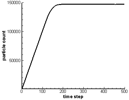
What makes particle storage fundamentally different from the mesh is that typically at the start of the simulation we have no idea how large the particle array needs to be. As an example, consider the simulation used to load an isotropic velocity. We start with an empty domain and inject particles from a point. The particles expand radially until they cross outside the computational domain. They are then removed from the simulation. The particle count will continue to grow until the number of particles created equals the number of particles lost through the boundaries. This is illustrated below in Figure 1, which comes from running the example program for 500 time steps. Since we do not know how many particles there will be at this steady state, we need a particle structure that can easily and efficiently grow to accommodate new particles.
Method 1: Single Memory Block
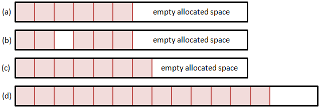
So let’s consider few alternatives. The first option is to use a single memory block. Here we allocate a particle array large enough to hold some initial estimated particle count. Whenever we need more space, we realloc the memory structure to expand it. But how do we add and remove particles? Removing any but the last particle will leave a hole in the list. We can leave this hole empty, and fill it the next time when adding a new particle. However, this approach is highly inefficient. Unless we create another data structure to hold the positions of all the holes, adding a particle will require us to loop through the entire list until we find an empty slot. The time required to add a particle thus directly depends on the number of particles, which is not something we desire. A somewhat better alternative is to shift the list forward to close the hole. Although we can now utilize memory copy operations, this approach will again get slower as the list size grows.
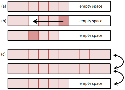
A much better alternative is to fill the hole right away with the last particle from the list and decrement the size of the list. This is shown in Figure 2. Unlike the data shifting method, this method rapidly closes the hole by rearranging the order of particles – the particle that was before last in the list may now end up somewhere in the middle. However, the PIC method (at least the way we implement it) is independent of the actual particle index in the list. This approach also assures that the list is free of holes, and thus new particle are always added to the end of the list. The add operation is now independent of the particle list size. One caveat with this approach is that we need to make sure to recheck the current position if the particle is removed, since post the removal, the current position will contain a new particle. Thus, if we are using a for loop, we need to decrement the current index prior to continuing,
for (p=0;p<np;p++)
{
    /*move particle*/
    remove = move(particles[p]);

    /*remove if needed*/
    if (remove)
    {
        copyPart(particles[p], particles[np-1]);
        np--;  /*decrement particle count*/
        p--;   /*recheck current position*/
    }
}
Method 2: Particle Block List
The above method used to be quite common and still is in legacy (Fortran) codes. But it has one significant disadvantage, especially when deployed on modern multitasking computers. As the particle count grows so does the requirement for a single large contiguous memory block. It may not be possible to get a block large enough even if the computer is reporting sufficient total RAM, due to memory fragmentation. As such, it is better to distribute the particle list to a number of blocks, each holding up to some prescribed number (such as 10,000) particles. Adding a particle requires looping over the blocks to find the first block with an empty space. The particle add is now no longer a fixed-time operation, but scales with the number of particle blocks. But since the number of blocks is relatively small (100 for one million particles and 10,000 particles per block), this overhead is also relatively small and can be further reduced by increasing the block size. This method is illustrated below in Figure 3.
Method 3: Linked List
The linked list is conceptually the simplest data structure for holding particles. In a linked list, particles are scattered through memory, and we don’t need to worry about needing a contiguous memory block. Particles can also be easily removed by breaking and rejoining the links,
part->prev->next = part->next;
part->next->prev = part->prev;
free(part);
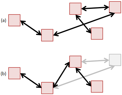
The issue with linked lists in general is that they are inefficient from the cache perspective. This was shown in the previous article on memory access. However, since a typical particle push operation requires access to a wide range of data structures, it is quite difficult to make the particle push cache friendly without going to great lengths in optimizing the rest of the code. As such, the fact that a linked list is not cache friendly gets lost when considering the bigger picture of gathering field variables or checking for surface impacts. All these operations will in general destroy the cache.
Timing Studies
When developing any scientific computing code, it is critical that you perform profiling studies to compare performance of a piece of code. Often, the solution that may appear to be the fastest won’t be so. Such is the case here. I compared the three methods above, and got the following times:
| Method | Time (sec) |
|---|---|
| Single Block | 24.42 |
| Part Block | 8.39 |
| Linked List | 7.36 |
Hence we can see that in this particular implementation, the linked list wins. These particular times come from a Java program in which we used the API ArrayList and LinkedList to hold the data. The Java implementation of the ArrayList performs something similar to what we described in the first half of Method 1. Instead of leaving a hole, the remove operation shifts the portion of the list after the removed entry forward to close the hole. As such, the remove operation performance scales directly with the size of the list, in a fashion analogous to the add with holes. This explains the large difference in times between this method and the rest. For the Particle Block method, we developed our own data structure that implements the basic functionality of the List and Iterable interfaces. This makes it very easy to change the data structure the code is using, simply uncomment the appropriate line on line 302,
//ArrayList<Particle> particles = new ArrayList<Particle>();
  LinkedList<Particle> particles = new LinkedList<Particle>();
//ParticleBlockList particles = new ParticleBlockList();
Source Code
You can download the entire source code here: ParticleSpeedTest.java.
By the way, these are just few of the many possible ways of storing particles. Furthermore, a linked list may not be fastest in your particular implementation. That’s why it’s important to do the profiling studies. I would be interested in hearing from you. What method do you use in your programs? Which have you found to be the fastest?
How about making a block containing all particles in a cell, so that it is efficient for MCC or DSMC collisions? In your speed test, how large is the block size? what size is the best? Thank you.
Right, but particles move in and out of the cell at each time step, so that may not really work.
Hi Lubos,
I think wphu above has a point. Consider this: each cell in a domain mesh has a pre-allocated particle list of size n (say, 100). Particle positions are by default stored as local coordinates within that cell. Events where a particle leaves the cell are immediately caught by negative local coordinates and handed over to the corresponding neighboring cell’s particle list. Could potentially work super smooth in unstructured meshes. What’s more, it could assist in join/split operations: when the pre-allocated particle list of a specific cell is already full upon entry of a new particle, some will be joined and the specific weight adjusted to make the list length n (=100) again. One could specify also a minimum list length upon which particles are split to adjust in the other direction. One could even think of pre-allocating particle list of sizes in relation to the specific cell’s volume.
What do you think?