Starfish Tutorial Part 3: Surface Interactions

Introduction
This is Part 3 of the five-part Starfish tutorial. In the previous step, we added a source to simulate the flow of ions over an infinitely long cylinder. When the ions collided with the cylinder, they were simply removed from the simulation. This is the default surface interaction that occurs if no other model is defined. It is not physically realistic. In reality, when low energy ions collide with a surface, they tend to pick up an electron from the surface and recombine into a neutral. In many plasma processes, surface recombination is the dominant plasma loss mechanism. Recombination in the gas itself is a three body process that is negligible at densities below 1e19 m-3. Although significantly lower than atmospheric pressure, this density is still several orders of magnitude higher than densities present in common space plasma applications. For instance, the ambient plasma density at the Low Earth Orbit is around 1e12 m-3. Plasma thrusters such as ion and Hall thrusters create plumes with densities in the range of 1e15 to 1e17 m-3.
Modeling Surface Interactions
In this tutorial, we will add surface recombination to our model. This is done via Starfish’s interactions module. This module handles reactions between all kinetic, fluid, and solid materials. We first create a new text file in the simulation directory called interactions.xml. The content of this file is
<!-- material interactions file -->
<material_interactions>

<surface_hit source="O+" target="SS">
<product>O</product>
<model>cosine</model>
<c_accom>0.5</c_accom>
<c_rest>0.9</c_rest>
</surface_hit>

</material_interactions>
and we load this file by adding
<load>interactions.xml</load>
to starfish.xml. We also need to add a new material to the database – remember, Starfish does not contain any built-in materials. We add the following to materials.xml:
<material name="O" type="kinetic">
<molwt>16</molwt>
<charge>0</charge>
<spwt>5e1</spwt>
</material>
We also tell the code to output neutral gas data by modifying the output command as follows:
<output type="2D" file_name="results/field.vts" format="vtk">
<scalars>phi, rho, nd.o+, nd.o</scalars>
<vectors>[efi, efj], [u.o+,v.o+], [u.o,v.o]</vectors>
</output>
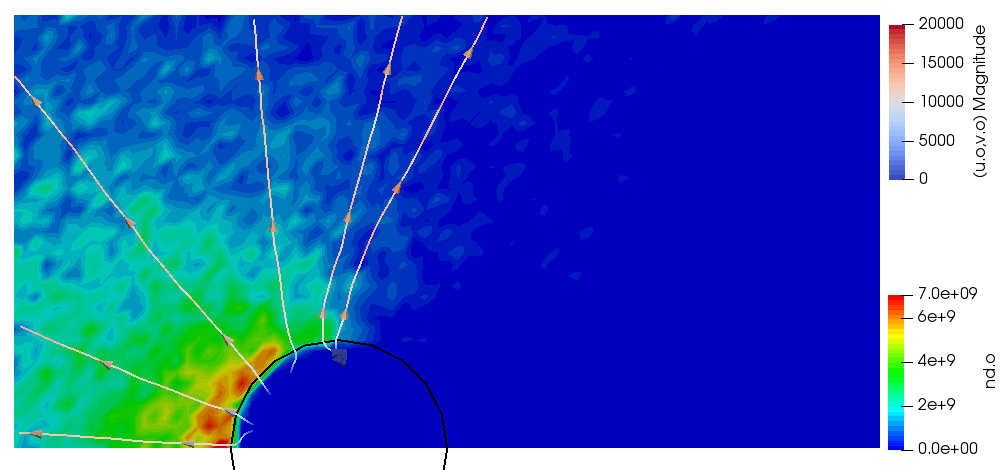
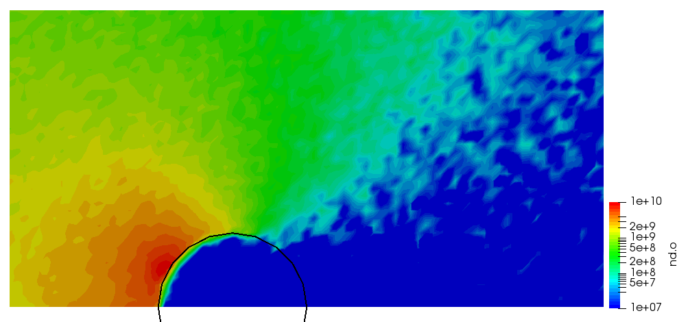
That’s it! You have just told the code to model surface recombination. If you run the simulation, you will get results similar to Figure 1 below.
Product Material Type
Let’s look through this step-by-step. The heart of this exercise is the material interaction. Each material interaction involves at least three participants: source, target, and product. The distinction between sources and products becomes blurry when dealing with collisions. However, they are clearly distinct when dealing with surface interactions. In this case, the source is the “flying” component. The target is the material that the source hits – the material from which the surface is made of. The product is the material the source turns into after undergoing the impact. In this case, we have told the code to turn O+ ions into O atoms after colliding with Stainless Steel surfaces.
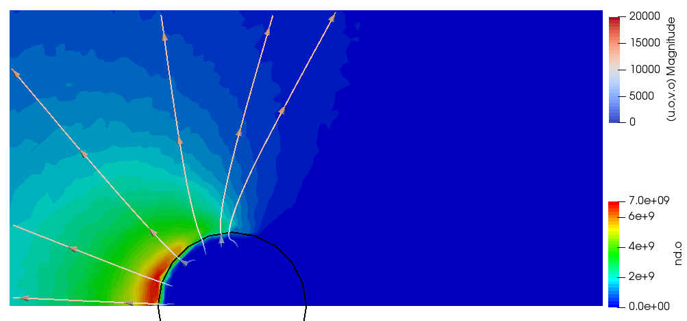
When you look in the materials file, you will see that the specific weight of the oxygen atoms (O), 5e1, differs from the specific weight of the oxygen ions (O+), 1e3. The code takes this into account, and creates, on average, 200 atom particles per each impacting ion. You can test this out yourself by changing the value and seeing the number of particles change. The actual density of oxygen atoms will stay the same, but the data will become noisier as the number of particles is reduced. This can be seen below in Figure 1.
We can also compare the particle counts from the screen output. With neutral weight of 5e1, we obtain:
it: 395	O+: 172097 O: 1091238
it: 396	O+: 172104 O: 1090858
it: 397	O+: 172106 O: 1091046
it: 398	O+: 172127 O: 1091258
it: 399	O+: 172153 O: 1091521
Processing <output>
Processing <output>
Processing <output>
Done!
and with 5e3 we get:
it: 395	O+: 172160 O: 11291
it: 396	O+: 172182 O: 11305
it: 397	O+: 172240 O: 11323
it: 398	O+: 172259 O: 11328
it: 399	O+: 172281 O: 11315
Processing <output>
Processing <output>
Processing <output>
Done!
As expected, the number of neutral simulation particles has dropped by two orders of magnitude.
Material Interaction Model
Getting back to the input file, so far we have only told the code to turn O+ into O. However, we have yet to specify how the new particles will leave the surface. This is done via the model field. Even relatively smooth surface will contain irregularities on the atomic scale. Furthermore, in many cases, incoming molecules do not bounce off the surface like a tennis ball. Instead, they momentarily settle on the surface and then they are re-emitted in a direction that tends to follow Lambert’s cosine law. The cosine model models this behavior. The angle of the emitted particle will scale proportionally to the cosine of angle between the velocity vector and the surface normal. Some additional models that are available include specular and diffuse (random) reflection.
Post-Impact Velocity
OK, so now we have specified the material and the direction, but we still need to specify the speed of the outgoing particles. This is done via the c_rest and c_accom coefficients. These correspond to the coefficient of restitution and the coefficient of thermal accommodation. The first controls the amount of incoming energy that is lost to the surface impact. At present, this energy is simply discarded, perhaps in the future a more advanced thermal model will include this in updating the surface temperature. It is given by
$$ c_{rest} = \dfrac{|v_{final}|}{|v_{initial}|}$$
Note that this assumes the surface is at rest.
The coefficient of thermal accommodation specifies the fraction of incoming particles that will completely forget their incoming velocity and will instead come off with a velocity corresponding to the thermal velocity of the surface. The overall algorithm is as follows:
/*magnitude of post-impact velocity due to coefficient of restitution*/
v_refl = vel*c_rest;

/*magnitude due to thermal accomodation*/
v_diff = SampleMaxwSpeed(target_temperature);
v_mag = v_refl + c_accom*(v_diff-v_refl);

/*create particle with velocity magnitude v_mag*/
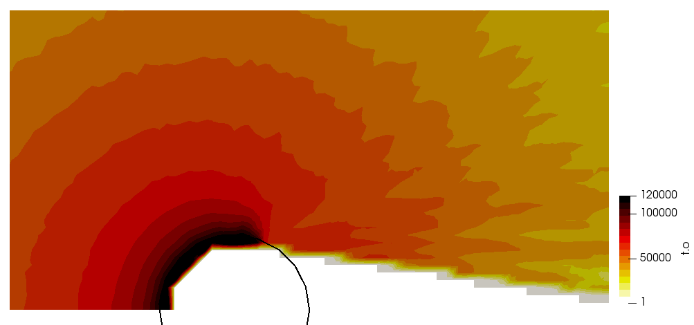
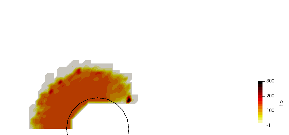
We can observe the effect of the coefficient of accommodation by visualizing the neutral temperature. With the default value of 0.5, the neutrals have a very large temperature due to neutrals bouncing off with half speed of the high velocity impacting ions. Note that this may not be a real “temperature” – the temperature is computed by assuming a Maxwellian VDF. With full thermal accommodation, the neutral temperature drops to the wall temperature specified in the boundary file.
Complex Interaction Types
The results from the above case were shown in Figure 1. We will now consider a more complex surface model. In the above example, all incoming ions turned into neutrals and were re-emitted. However, Starfish also allows you to define multiple interaction types with a prescribed probability of occurrence. As an example, let’s consider a more complex interactions file:
<!-- material interactions file -->
<material_interactions>

<!-- cosine law, 40% of particles -->
<surface_hit source="O+" target="SS">
<product>O</product>
<model>cosine</model>
<prob>0.4</prob>
<c_accom>0.5</c_accom>
<c_rest>0.9</c_rest>
</surface_hit>

<!-- specular reflection, 20$ of particles -->
<surface_hit source="O+" target="SS">
<product>O</product>
<model>specular</model>
<prob>0.2</prob>
<c_accom>0</c_accom>
<c_rest>1.0</c_rest>
</surface_hit>

</material_interactions>
This file is similar to the one from above, except that now we have specified two surface_hit fields. In addition, we added a new field called prob. This field gives the probability for this model. As you can see, these two probabilities add up to a value less than 1.0. This is OK, the remaining particles will be handled by default handler, one that absorbs incoming particles. The resulting plot from this simulation is shown below in Figure 3. It is quite similar to the one from above, but the density of neutrals has decreased correspondingly.
Continue onto Part 4.
Hey,
could you please give a reference to the following statement in this article:
“Recombination in the gas itself is a three body process that is negligible at densities below 1e19 m^-3”.
Thanks a lot,
Johannes Peter
Hi Johannes,
The first part of the statement arises from the chemical reaction, i.e. \(A + e \to A^+ + e + e \) for impact ionization. Recombination is the reversal of this process and the third body is needed to absorb the additional energy. Jahn goes into a lot of detail on the various chemical processes occurring in plasmas in the electric propulsion devices.
The second part is coming from my own experience when modeling Xenon ion thruster plumes. I don’t remember right now off the top of my head what recombination relationship I was using back then, but the recombination rate came out to be negligible (below fraction of a percent) at the densities below 1e19 #/m^3. I’ll try to dig up some relationships and get back to you.