CTSP Molecular Contamination Modeling Validation

This article summarizes validation effort for the molecular transport algorithms in our contamination simulation program CTSP. The idea is that this post will grow in time as more validation studies are completed.
Conductance
The first validation study was made to model conductance through a cylindrical tube. The tube was sketched and meshed in Salome and exported in UNV format. The tube consists of three sections: inlet, body, and outlet. An initial 1e-10 thick surface layer was specified on the inlet. The inlet temperature was set warm enough such that the entire surface layer desorbed on the first time step. Temperature of the body was set to the same temperature as the inlet, preventing any impacting molecules from adsorbing. Instead, these molecules bounce off following the cosine (Lambertian) law, which is the primary target of this validation study. The temperature on the outlet is set to zero so that impacting molecules stick. One remaining issue is dealing with adsorption on the inlet. We are interested in also capturing molecules that bounce “back” and leave through the inlet. To do this, a sticking coefficient is defined on the inlet. This coefficient overrides adsorption probability from the surface temperature. It can be used to model UV photo-polymerization, where molecules stick to a surface exposed to UV light, even if the surface is not cold enough to warrant deposition otherwise. CTSP input file for this simulation is listed below.
#load surface
surface_load_unv{file_name:"tube4.unv",view:1,units:mm}

#materials
solid_mat{name:al, mass: 100}
gas_mat{name:hc1, mass: 94, spwt: 1e14, Ea:12, C:10, r:1.55e-10}

#define components, surface height in monolayers
comp{name:g_inlet, mat:al, trapped_mass:1e-2, trapped_mat:[0*hc1], surf_h:1e-10, surf_mat:hc1, temp:350, c_stick:1.0}
comp{name:g_body, mat:al, trapped_mass:0,surf_h:0,temp:350}
comp{name:g_outlet, mat:al, trapped_mass:0,surf_h:0,temp:0}	#set cold so everything sticks

#enable outgassing
source_outgassing{}

#save results
surface_save_vtk{skip:25,file_name:"tube"}
particle_save_vtk{skip:25,file_name:"particles"}

#run simulation
ctsp{dt:5e-5,nt:10000,diag_start:1,diag_skip:5}
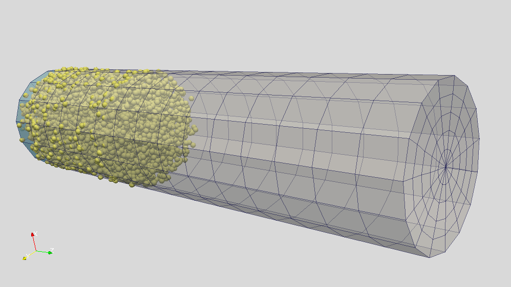
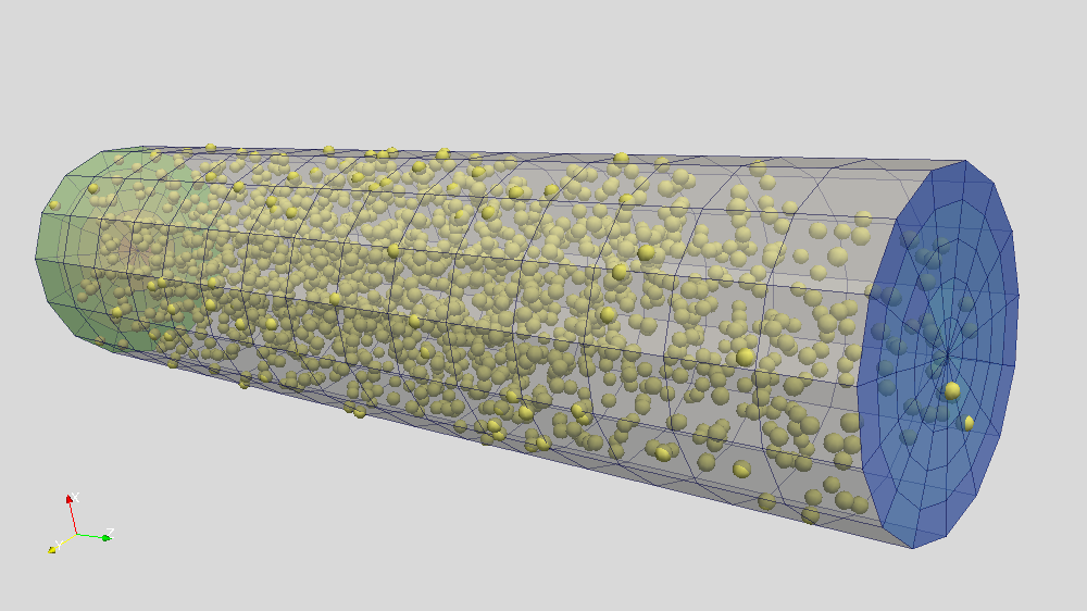
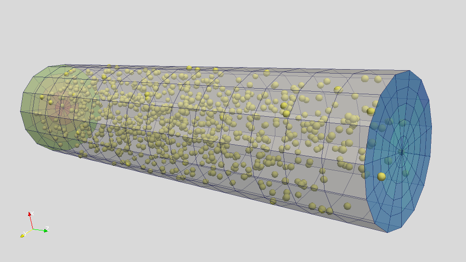
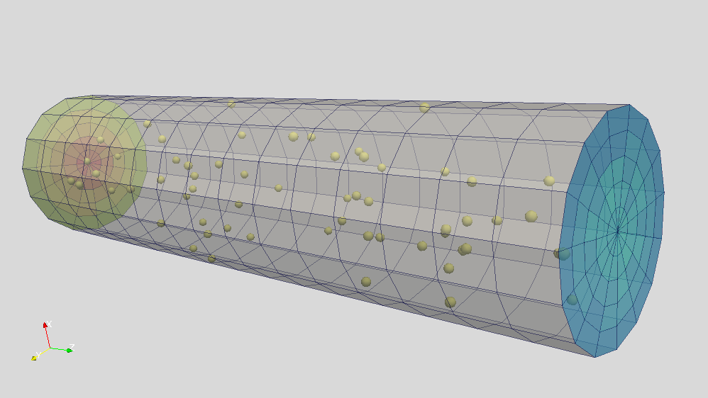
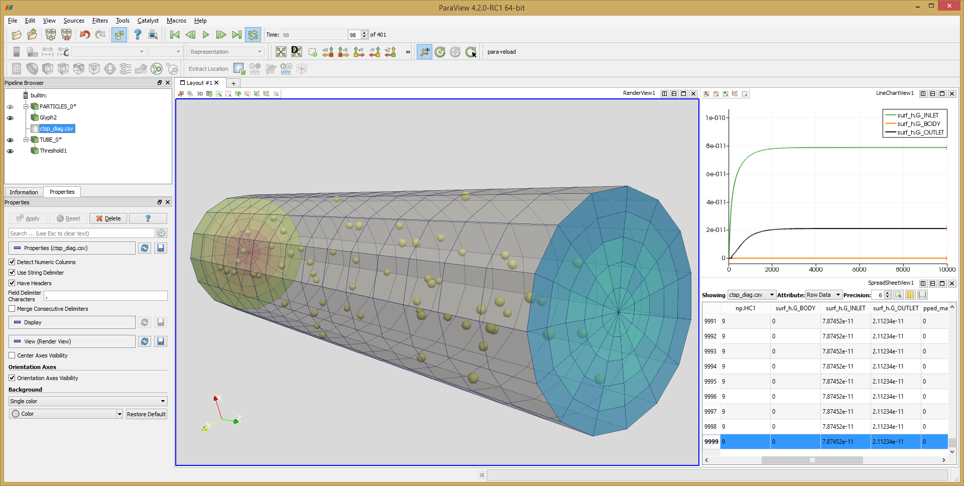
Figure 1 below shows several snapshots from the simulation. Outputting particle positions is not actually needed, but the ability to do so is one neat feature of CTSP, as it uses DSMC/PIC-like algorithm and pushes multiple particles concurrently. The simulation continues until all particles are absorbed. The plots were generated using Paraview. Figure 2 shows a screen shot of Paraview also displaying line plots of surface layer thickness versus time. This plot lets us see that the simulation has reached steady state.
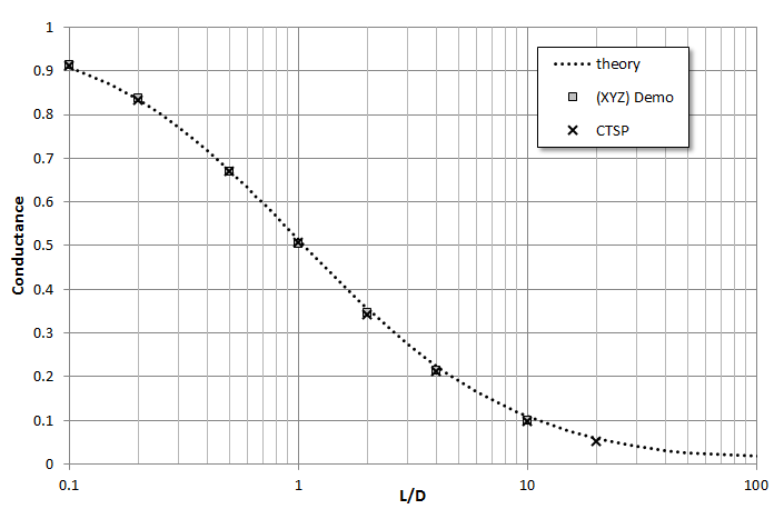
Finally, Figure 3 summarizes the computed conductance values for several different tube L/D ratios. These are compared to data from O’Hanlon [1]. These results are also compared to a stand-alone cylindrical tube conductance code that will be posted on the blog soon. It can be seen that CTSP and the stand-alone code agree well with theory but there is a small common discrepancy shared by the two codes. They both slightly over-estimate conductance for smaller L/D ratios, while underestimating it for larger L/D values. Perhaps these issues are just due to an insufficient number of particles? The simulations used about 30k particles for the smaller L/D ratios, and about 200k for the L/D of 10 and 20. Still, the discrepancy is quite small to let me claim that the code passed this test.
Outgassing Rate
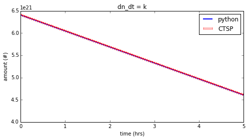
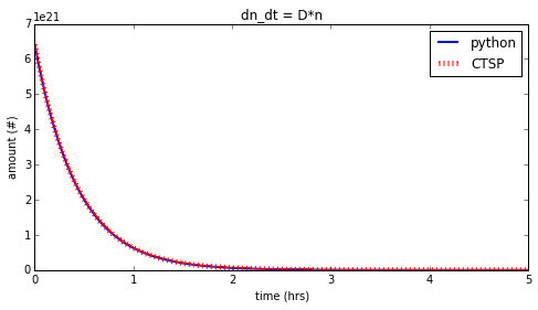
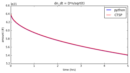
CTSP currently supports three models for the outgassing rate: 1) const with \(dN/dt = k\), 2) kn where \(dN/dt = C_0exp(-E_a/RT)N\), and 3) sqrtt with \(dN/dt = C_0exp(-E_a/RT)N/\sqrt{t}\). The last model is the default, and corresponds to equation 2-18 in [2]. This comparison simply tested the implemented integration. The three above equations were coded up in Python, and mass remaining versus time from Python was plotted against the results from CTSP. The results are shown below, showing agreement.
References:
[1] O’Hanlon, J.F., A User’s Guide to Vacuum Technology, Wiley-Interscience, 3rd edition, 2003
[2] Tribble, A.C, Fundamentals of Contamination Control, SPIE Press, 2000