Free molecular flow in a cylindrical pipe – with multithreading

 You may have noticed many recent blog posts dealing with “contamination modeling”. While I started my scientific computing career with plasma simulations, these days much of my focus (and work projects) is spent on modeling contaminant transport. It’s like PIC, but without all the complicated plasma physics! There are two types of contaminants that are of interest: molecular and particulate. When it comes to molecular transport, designer of some sensitive sensor may want to know how much deposition to expect when placed in a vacuum chamber. Coming up with the answer requires computing gray body view factors between the target and all sources of contaminants. There are two ways of going about this: solving a system of linear equations, or performing Monte Carlo ray tracing. The ray tracing approach shares many similarities with PIC: we use sources to inject simulation particles, integrate their positions, perform surface interactions, and compute surface flux to objects of interest.
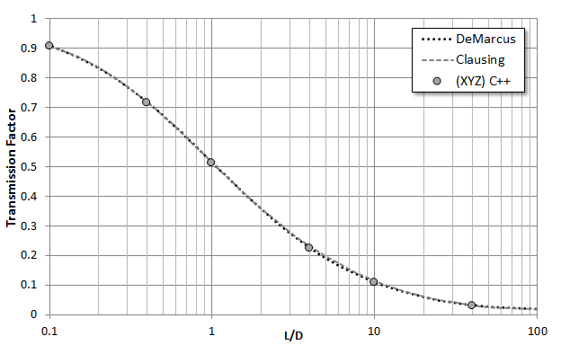
While this sounds simple, the devil is in the details. In this case, the detail is the surface interaction. The sensitive component will often be located outside a direct line of sight of sources, and it may take a molecule many bounces before it randomly finds its way to the sensor. Hence it is crucial that your code models these bounces correctly. Molecules reflecting from a rough surface bounce off such that flux follows cosine distribution about the surface normal. It’s quite easy to implement this diffuse reflection incorrectly! A common test is to consider conductance, or specifically transmission probability, of molecules through a cylindrical pipe. This problem was first addressed by Clausing (in 1932!). Clausing [1] tabulated his closed form formula for several simple geometries, including a pipe of varying L/D (length over diameter) ratios. Other researchers later came up with their own values for the “Clausing factor”, including DeMarcus and Berman. This latter data is tabulated in O’Hanlon [2]. The two solutions are very close but diverge slightly once L/D exceeds 5, as can be seen in Figure 1.
Simulation Code
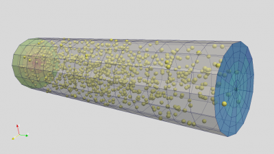
In this article we’ll write a code for computing these transmission factors for free molecular flow in a cylindrical pipe. The pipe is defined analytically (as opposed to using a surface mesh), allowing us to consider arbitrary L/D ratios. The diameter D is set to 1, hence we simply vary the pipe length L. The pipe consists of three surfaces: inlet, wall, and outlet. The simulation proceeds as follows:
- Particles are continuously injected at the inlet at random position and velocity following the cosine law
- If a particle hits the wall, it is reflected from the point of impact with new velocity also sampled from the cosine law
- If a particle crosses the inlet or the outlet, the particle is removed and the appropriate counter inlet or outlet is incremented
- Simulation runs for a total of million time steps. Transmission factor is computed as outlet/(inlet+outlet)
The main loop is shown below:
    /*main loop, runs for num_ts time steps*/
    void mainLoop()
    {
        for (ts=0;ts<num_ts;ts++)
        {
            InjectParticles();
            MoveParticles();
        }

        finished = true;
    }
Below is the code for injecting particles. It uses lambertianVector function to sample a random unit vector about normal with the two tangents given by tang1 and tang2.
    /*injects np_per_ts particles at z=0 with cosine distribution about z axis*/
    void InjectParticles()
    {
        double source_n[3] = {0,0,1};     //source normal direction
        double tang1[3] = {1,0,0};        //tangent 1
        double tang2[3] = {0,1,0};        //tangent 2

        for (long p=0;p<np_per_ts;p++)
        {
            double pos[3];
            double vel[3];
            double rr;

            //select random position between [-R:R]x[-R:R], accept if in tube
            do {
                pos[0]=R*(-1+2*rnd());
                pos[1]=R*(-1+2*rnd());

                rr= pos[0]*pos[0]+pos[1]*pos[1];
                if (rr<=R*R) break;
            } while(true);

            pos[2]=0;    //z=0

            //velocity
            double n[3];
            lambertianVector(n,source_n,tang1,tang2);

            //multiply by drift velocity
            vel[0]= n[0]*vdrift;
            vel[1]= n[1]*vdrift;
            vel[2]= n[2]*vdrift;

            //add to dynamic storage
            particles.push_back(new Particle(pos,vel));
        }
    }
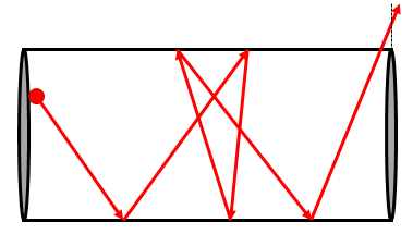
The particle mover is shown below. Particles are stored in a C++ linked list data structure. This data structure makes it easy to remove entries (killed particles) but is not as efficient to traverse as the consecutive array. We iterate through the particles using an iterator. Erasing a particle returns a new iterator and invalidates the existing one, hence the need for the while loop. The iterator is incremented for alive particles with it++. The code structure should be familiar to anyone having taken my PIC Fundamentals course. We check for wall impact by computing \(r=\sqrt{x^2+y^2}\). If \(r>R\), the cylinder radius, the particle hit a wall. We also check for particles leaving through inlet or the outlet by making sure that \(z\in(0,L)\). We check for wall impact first, otherwise the particle in the sketch above may be counted as leaving the tube on the final bounce. If a particle hit the wall, the parametric position of the impact is computed from t=(R-r0)/(r-r0) where r0 is the radial distance of the particle at the start of the push. The particle is then pushed for the remaining dt_rem.
    /*moves particles, reflecting ones hitting the tube wall*/
    void MoveParticles()
    {
       double x_old[3];

       list<Particle *>::iterator it = particles.begin();
       double sum=0;

       while (it!=particles.end())
       {
           Particle *part = *it;
           double dt_rem = dt;

           //while there is delta t left in particle push
           while(dt_rem>0)
           {
               //save old position
               vec::copy(x_old,part->pos);

               //new position, x = x + v*dt
               vec::mult_and_add(part->pos,part->pos,part->vel,dt_rem);

               //did particle hit the wall?
               double rr = part->pos[0]*part->pos[0]+part->pos[1]*part->pos[1];
               if (rr>=R*R)
               {
                   //compute intersection point
                   double r = sqrt(rr);
                   double r0 = sqrt(x_old[0]*x_old[0]+x_old[1]*x_old[1]);
                   double t = (R-r0)/(r-r0);

                   //push particle to the wall
                   vec::mult_and_add(part->pos,x_old,part->vel,t*dt_rem);

                   //update remaining delta_t
                   dt_rem -= t*dt_rem;

                   //surface normal vector
                   double normal[3];
                   normal[0] = 0-part->pos[0];
                   normal[1] = 0-part->pos[1];
                   normal[2] = 0;

                   vec::unit(normal,normal);

                   //get tangents
                   double tang1[3], tang2[3];
                   tangentsFromNormal(normal,tang1,tang2);

                   //cosine emission
                   double dir[3];
                   lambertianVector(dir, normal, tang1, tang2);
                   for (int i=0;i<3;i++)
                       part->vel[i]=dir[i]*vdrift;
               } //dt_rem
               else //no wall impact
               {
                    //particle left through inlet or outlet?
                   if (part->pos[2]<=0 || part->pos[2]>=L)
                   {
                       if (part->pos[2]<0)
                           inlet++;
                       else
                           outlet++;
                       //kill particle
                       delete part;
                       it = particles.erase(it);
                       break;        //break out of dt_rem loop
                   }
                   else    //particle inside the cylinder
                   {
                       dt_rem = 0;
                       it++;    //go to next particle
                   }
               }
           } //while dt_rem
       }    //particle loop
    }
Below is the “meat” of the simulation, the code that samples a random vector according to the cosine law.
    /*returns direction from cosine distribution about normal given two tangents*/
    void lambertianVector(double dir[3], double normal[3], double tang1[3], double tang2[3])
    {
        //sample angle from cosine distribution
        double sin_theta = sqrt(rnd());     //sin_theta = [0,1)
        double cos_theta = sqrt(1-sin_theta*sin_theta);

        //random rotation about surface normal
        double phi = 2*PI*rnd();

        double vn[3],vt1[3],vt2[3];
        vec::mult(vn,normal,cos_theta);
        vec::mult(vt1,tang1,sin_theta*cos(phi));
        vec::mult(vt2,tang2,sin_theta*sin(phi));

        //add components
        for (int i=0;i<3;i++)
            dir[i] = vn[i]+vt1[i]+vt2[i];
    }
The lambertianVector function requires besides the normal also two tangents. For a cylinder, there is probably a closed form for the tangents. However, the below code also works. It creates two randomly oriented tangent vectors from an arbitrary normal. It does this by first finding the spatial direction in which the normal has the largest component. It then creates a test vector in the “following” direction. As I am not using the right syntax, I am sure this is quite confusing. If the normal is mainly in the y direction, the test vector will be in the z direction. The two vectors are then crossed, giving us the first tangent, since the result of a cross-product is perpendicular to the two arguments. The second tangent is computed by crossing the first tangent with the normal.
    /*generates two tangent vectors, assumes normalized input*/
    void tangentsFromNormal(double n[3], double tang1[3], double tang2[3])
    {
        //get maximum direction of the normal
        int max_i=0;
        double max = abs(n[0]);
        for (int i=1;i<3;i++) if (abs(n[i])>max) {max=abs(n[i]);max_i=i;}

        //create a test vector that is not parallel with norm
        double test[3] = {0,0,0};
        if (max_i<2) test[max_i+1]=1.0; else test[0]=1.0;

        //cross the two vectors, this will give the first tangent -perpendicular to both
        vec::cross(tang1,n,test);    //assuming n is already normalized

        //and the second vector//
        vec::cross(tang2,n,tang1);
    }
Multithreading
In order to get reasonable results we need to simulate a large number of test particles. Since we are modeling free molecular flow, the particles don’t influence each other in any way. As such, we could trace each particle from start to finish before moving on to the next one, or push them all concurrently through small time steps as is done here. This also means that this code is embarrassingly parallel. In the previous post I showed you how to use graphics cards (GPUs) to parallelize plasma codes. In this post, I show you how to use multithreading. All modern CPUs contain multiple cores. For instance, my fairly mid-range laptop from 2014 features the Intel i7-4700HQ CPU. This CPU contains 4 cores and supports 8 concurrent executing threads. This means that instead of pushing just one set of particles at once, we can push more of them, theoretically up to eight. Multithreading is one of the main three ways of achieving parallelization that will be covered in the Distributed Computing course. It’s a shared memory approach, where bunch of simulations are running on the same system and thus have access to the same memory. C++11 natively supports multithreading with #include <thread>. This defines a std::thread object. Launching a new thread is quite trivial; we simply use syntax like std::thread(function, params), which will launch function(params) as a new thread. Such an approach works fine for simple functions. However, here we need to encapsulate data needed by each thread. In order to avoid data contention, we let each thread have its own set of particles. We also need each thread to have its own random number generator, since only one thread can access a generator at a time. Our data in encapsulated in a class called ConductanceXYZ. The listing is shown below. The mainLoop also belongs to this class and was discussed previously. Note how the constructor generates a new thread. The thread calls a static function start which is passed a ConductanceXYZ class pointer. The function then simply launches mainLoop in that class.
/*conductance class*/
class ConductanceXYZ
{
public:
    const double R=0.5;      //cylinder radius
    const double L;          //cylinder length

    const long np_per_ts;    //number of particles to create per time step
    const int num_ts;        //number of timesteps to run

    const double vdrift = 5;    //injection velocity
    list<Particle*> particles;  //list of particles

    const double dt=1e-2;    //simulation time step size
    int ts;        //current time step

    int inlet = 0;    //number of particles crossing inlet
    int outlet = 0;   //number of particles crossing outlet

    bool finished = false;    //set true once loop finishes

    /*constructor, initializes parameters and seeds random number generator*/
    ConductanceXYZ(double L, long np_per_ts, int num_ts):
        gen((unsigned int)chrono::system_clock::now().time_since_epoch().count()),
        L(L), np_per_ts(np_per_ts), num_ts(num_ts)    {
        thr = new thread(start, this);
    }

    thread *thr;
    /*thread start*/
    static void start(ConductanceXYZ *p)   {p->mainLoop();}

    /*random number generator*/
    mt19937 gen;
    double rnd() {
        uniform_real_distribution<double> rnd_dist(0.0,1.0);
        return rnd_dist(gen);
    }
//	...
}
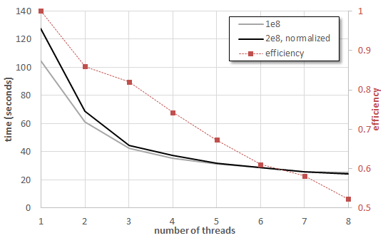
Below is the main function where everything starts. We first query the system for the number of supported concurrent threads. This becomes the default value, although it will severely slow down your computer as it prevents the operating system from running its own threads. We then use optional command line arguments to set the cylinder length and also the total number of simulation particles. The particle count per thread is then computed. Finally we compute the number of particles per thread per time step, np_per_ts. This value is floored at 1, meaning that the code will always generate at least 1 million (num_ts) particles per thread. We then create num_threads ConductanceXYZ classes and store these in a linked list. At this point, the main function doesn’t know that there are these other simulations running. If we don’t do anything else, the code would shortly terminate. Hence we need to add a do-while loop that keeps main alive while the threads are still running. The way we check is by first setting bool finished=true. Each thread has its own finished boolean which will be false while the time step loop is running. As we iterate through the threads, we perform a boolean “and”, finished &= sim.finished. Any non-true value will clear the boolean. We also reduce the inlet and outlet counters into a single global value. We use this to compute the transmission factor. As you can see in Figure 1, the results are quite good (there is a <1% error using 1e7 particles). But what about parallel performance? This is plotted below in Figure 2. Two cases are plotted: 1e8 and 2e8 particles. Times for the 2e8 case were divided by two to allow us to compare the trends. I thought that perhaps the efficiency will improve with a larger number of particles on more threads, but that was not the case. We can see that there is a huge improvement from 2 to 4 threads. However going past 4 threads doesn’t really bring much more speedup. With 8 threads, the parallel efficiency is only about 50%, meaning the code is running the same speed as a 100% efficient 4 threaded code (our code is however only about 74% efficient with 4 threads). There are probably multiple reasons for this. My system has only 4 cores, so the other 4 threads are probably some non-physical virtual threads. Also, I was running this on Windows with many applications opened, meaning there were many other processes competing for CPU time.
#include <iostream>
#include <iomanip>
#include <thread>
#include <random>
#include <list>
using namespace std;
//...

/*********   MAIN *********/
int main(int nargs, char*args[])
{
  int num_threads = thread::hardware_concurrency();
  cout<<"Number of supported concurrent threads: "<<num_threads<<endl;

  double L=1;
  double part_totf = 1e7;	//double so we can use scientific notation

  //get parameters from command line if specified
  if (nargs>1) L=atof(args[1]);
  if (nargs>2) num_threads=atoi(args[2]);
  if (nargs>3) part_totf=atof(args[3]);

  //show active parameters
  cout<<"L = "<<L<<"\tnum_threads = "<<num_threads<<"\tpart_tot = "<<part_totf/1e6<<"mil"<<endl;

  long part_tot = (long)part_totf;
  int num_ts = 1000000;	//number of time steps
  long part_per_thread = (long)(part_tot/((double) num_threads)+0.5);

  long np_per_ts = (long)(part_per_thread/(double)num_ts+0.5);
  if (np_per_ts<1) np_per_ts=1;	//make sure we get at least 1

  clock_t start = clock();    //start timer

  list<ConductanceXYZ> sims;    //storage for our simulations

  //create num_threads simulations
  for (int i=0;i<num_threads;i++)
      sims.emplace_back(L,np_per_ts, num_ts);

  //wait for threads to finish
  bool finished;
  do
  {
       long tot_gen = 0;
       long tot_out = 0;
       long tot_np = 0;
       int ts = num_ts+1;
       finished = true;
       //combine counts across threads and also check for completion
       for (ConductanceXYZ &sim:sims) {
            tot_gen += sim.inlet + sim.outlet;
            tot_out += sim.outlet;
            tot_np += sim.particles.size();
            if (sim.ts<ts) ts=sim.ts;
            finished &= sim.finished;    //boolean and, any false will clear it
       }
       double K=0;
       if (tot_gen>0) K=tot_out/(double)(tot_gen);
         cout<<"it="<<ts<<"\t np="<<setprecision(4)<<tot_np<<"\t K="<<K<<endl;

       //sleep for 50 milliseconds
       this_thread::sleep_for(chrono::milliseconds(50));
    } while (!finished);

  clock_t end = clock();
  cout<<"Simulation took "<<(end-start)/((double)CLOCKS_PER_SEC)<<" seconds"<<endl;
  return 0;
}
Source Code
You can download the code here: conductance.cpp. If using gcc, you need to compile with std=c++ flag. You can specify optional command line parameters L num_threads num_particles, for instance conductance.exe 0.4 4 1e7.
One note, if you are using Windows, do not run this under Cygwin. Cygwin still does not appear to support multithreading (if you know otherwise, let me know!). When running the code using GCC under Cygwin, I saw no improvement with multiple threads.
References
[1] Clausing, P, “The Flow of Highly Rarefied Gases through Tubes of Arbitrary Length”, Ann. Physik, (5) 12, 961, 1932
[2] O’Hanlon, J. F. A User’s Guide to Vacuum Technology, Wiley-Interscience, 2003