Brief Intro to GPU PIC with CUDA

GPU scientific programming has been all the craze the past few years. Early reports indicated possible speed ups between 10 and 100 times by moving computations to the graphics card. Who wouldn’t like that? A highly cited paper (by people at the CPU manufacturer Intel so some bias to be aware of!) showed that a more realistic improvement is closer to 2.5x. That’s less than 100x, but it’s still not something to completely blow off. Your system may be like mine in that it already has a graphics card that just ends up sitting idle most of the time. We may as well put it to use! In this article we will develop a simple 1D sheath PIC simulation using the NVIDIA CUDA language extension. The code is completely unoptimized, it doesn’t make use of fast memory types available on the GPUs, and in fact does most computation using double precision which the GPUs are not optimized for. The code also took only about two hours to write. Yet, it still outperforms the CPU version by almost a factor of two for large particle counts! This is what I wanted to show you in this article: getting the order of magnitude speed up on a GPU may be hard. But even without all that hard work, using just few simple steps, you may still be able to get a factor of two improvement, which is not bad at all.
GPU vs CPU model
GPUs are basically the vector supercomputer mainframes of days past squeezed into a tiny package. While a CPU can perform a single computation extremely fast, GPUs perform hundreds of computations in parallel with each taking longer than on the CPU. Consider the vector addition, for (int i=0;i<N;i++) a[i] = b[i] + c[i]. Ignoring compiler optimization and SIMD support in modern CPUs, the CPU version would first compute a[0] = b[0] + c[0], then move on to a[1] = b[1] + c[1] and so on. The GPU version on the other hand computes many of these sums concurrently. For instance, a[0:500] = b[0:500] + c[0:500] may be evaluated in parallel. This also shows that GPU computing mainly makes sense if the order of operations is not relevant. It would be more difficult to take advantage of vector architecture if each loop iteration depended on the previous result, as in for (int i=1;i<N;i++) a[i] = a[i-1] + b[i].
PIC Algorithm
So how does this relate to plasma simulations with the particle in cell method? PIC basically consists of two steps: 1) compute potential and electric field and 2) push particles. While both of these steps are candidates for parallelization (iterative field solver basically boils down to a fast matrix-vector math), in this article we only focus on the second item.
Think of a typical particle push algorithm:
for each particle in an array:
    gather electric field at particle position
    use electric field to update velocity
    use the new velocity to update position
There is nothing magical about how particles are ordered in the array. Whether we first push particle[0] before particle[1] or access the entries completely randomly, the results won’t change (but performance may go down for the random access). The particle push algorithm is thus a good candidate for off-loading to the GPU.
One Dimensional Sheath Code on a CPU
And this is exactly what is done in this code. We start with a simple fully-kinetic (electrons and ions treated as particles) one dimensional sheath simulation. The code is similar to the one developed in PIC Fundamentals, so please sign up for the course for more details. But there is one added handicap. The sheath simulation begins with the code loading uniform ion and electron density. As particles hit the wall, they undergo recombination, and are removed from the simulation. The original sheath code accomplished this by filling the gap created by the “killed” particle by the last entry. The number of simulation particles thus decreases with time. This type of reordering is however not straightforward to implement on the GPU. The CPU code was thus modified to just flag dead particles and skip over them in the loop. This handicap results in a 10% slow down. Instead of
if (part->x < domain.x0 || part->x >= domain.xmax) {
    /*replace this particle slot with last one*/
    part->x = species->part[species->np-1].x;
    part->v = species->part[species->np-1].v;
    species->np--;	/*reduce number of particles*/
    p--;	/*decrement to recompute this slot*/
}
we now have
if (part->x < domain.x0 || part->x >= domain.xmax) {
    /*mark particle as dead*/
    part->alive = false;
    species->np--;
}
GPU version
We will now develop the GPU version of the particle push, sheath-gpu.cu. The code uses the NVIDIA CUDA language extension set and as such you will need the developer kit plus a CUDA-compatible graphics card. The developer kit contains a special compiler called nvcc which generates the code for the GPU. If you are using Visual Studio on Windows, you can also download Nsight, which integrates CUDA development tools into the IDE. That was my setup, and this example was actually run through Visual Studio.
Initialization
First, we need to include few additional header files. We also define a simple error handler. It simply checks the status code returned by CUDA functions and terminates the program if an error occurred.
#include "cuda_runtime.h"
#include "device_launch_parameters.h"

/*CUDA error wraper*/
static void CUDA_ERROR( cudaError_t err)
{
    if (err != cudaSuccess) {
        printf("CUDA ERROR: %s, exiting\n", cudaGetErrorString(err));
        exit(-1);
    }
}
We start our main program by showing some basic information about the graphics card and then select the first card as the one to use. In a system with multiple cards, you may want to use results from the device query to find the one best suitable and use that one.
/* --------- main -------------*/
int main()
{
    /*get info on our GPU, defaulting to first one*/
    cudaDeviceProp prop;
    CUDA_ERROR(cudaGetDeviceProperties(&prop,0));
    printf("Found GPU '%s' with %g Gb of global memory, max %d threads per block, and %d multiprocessors\n",
        prop.name, prop.totalGlobalMem/(1024.0*1024.0),
        prop.maxThreadsPerBlock,prop.multiProcessorCount);

    /*init CUDA*/
    CUDA_ERROR(cudaSetDevice(0));
On my laptop, this line outputs: Found GPU 'GeForce GTX 860M' with 2048 Gb of global memory, max 1024 threads per block, and 5 multiprocessors.
Algorithm
The GPU cannot directly access the main system memory. Instead, the card contains its own data storage called global memory. This is just one of several different storage types available on a GPU. Of all these, global memory is the slowest. But it is also the only one we will use in our application. Global memory is the easiest to use. It is also accessible to all threads, and more importantly, can be used to communicate data between the CPU and the GPU.
Memory access is one of the major performance bottlenecks in a GPU application. Reviewing memory access would be a good “future work” project. But the objective of this example was to show that even without much effort we can still gain performance by using the GPU. Now having said that, it’s also important not too do anything particularly stupid. Since memory access is slow, it makes sense to do it as little as possible. Hence, we move the particles to the GPU at the start of the simulation and leave them there. Since our potential solve is done on the CPU side, we need the updated number densities. As is typical of PIC codes, our simulation contains many more particles than mesh nodes. Instead of copying millions of particles back and forth, we let the GPU reduce the particles positions, and then copy just the 100 floating point values corresponding to densities on the nodes of the simulation mesh. These are then used to compute plasma potential and electric field on the CPU. The electric field is then copied to the GPU.
A simplified version of the algorithm becomes:
a) C2G: Copy particles to the GPU
--Main Loop
1) GPU: Update particle positions
2) GPU: Compute density
3) G2C: Copy density from GPU to CPU
4) CPU: Compute potential and electric field
5) C2G: Copy electric field to the GPU
--
Moving Particles to the GPU
We could save main system memory by simply creating particles on the GPU. But to keep things simple, we initialize the particles on the CPU and then copy them to the graphics card. This means we need a double memory storage, one on the CPU and one on the GPU. This allocation is shown below. We allocate system memory using new and use cudaMalloc to allocate GPU global memory.
/*set material data*/
ions.mass = 16*AMU;
ions.charge = QE;
ions.spwt = PLASMA_DEN*domain.xl/NUM_IONS;
ions.np = 0;
ions.np_alloc = NUM_IONS;
ions.part = new Particle[NUM_IONS];
CUDA_ERROR(cudaMalloc((void**)&ions.part_gpu,NUM_IONS*sizeof(Particle)));

electrons.mass = ME;	// electrons
electrons.charge = -QE;
electrons.spwt = PLASMA_DEN*domain.xl/NUM_ELECTRONS;
electrons.np = 0;
electrons.np_alloc = NUM_ELECTRONS;
electrons.part = new Particle[NUM_ELECTRONS];
CUDA_ERROR(cudaMalloc((void**)&electrons.part_gpu,NUM_ELECTRONS*sizeof(Particle)));
We then load NUM_IONS and NUM_ELECTRONS uniformly distributed ions and electrons. Particle data is copied using cudaMemcpy. Note the last parameter, cudaMemcpyHostToDevice, telling the function we are copying from the host (the CPU) to the device (the GPU).
/*now do the same for electrons*/
double delta_electrons = domain.xl/NUM_ELECTRONS;
double v_the = sqrt(2*K*ELECTRON_TEMP*EV_TO_K/electrons.mass);
for (p=0;p<NUM_ELECTRONS;p++)
{
	double x = domain.x0 + p*delta_electrons;
	double v = SampleVel(v_the);
	AddParticle(&electrons,x,v);
}

/*copy particles to the GPU*/
CUDA_ERROR(cudaMemcpy(ions.part_gpu,ions.part,NUM_IONS*sizeof(Particle),cudaMemcpyHostToDevice));
CUDA_ERROR(cudaMemcpy(electrons.part_gpu,electrons.part,NUM_IONS*sizeof(Particle),cudaMemcpyHostToDevice));

/*CPU particle memory could be deleted now as it's not needed anymore*/
What’s important to point out is that part_gpu acts as a regular pointer, but it is pointing to memory not accessible by the CPU. We will need to pass this pointer to our GPU code so it knows where to find particles.
GPU Particle Push
Below is the code used to push particles in the CPU version
/* moves particles of a single species*/
void PushSpecies(Species *species, double *ef)
{
    /*precompute q/m*/
    double qm = species->charge / species->mass;

    /*loop over particles*/
    for (int p=0;p<species->np_alloc;p++)
    {
        /*grab pointer to this particle*/
        Particle *part = &species->part[p];

        if (!part->alive) continue;

        /*compute particle node position*/
        double lc = XtoL(part->x);

        /*gather electric field onto particle position*/
        double part_ef = gather(lc,ef);

        /*advance velocity*/
        part->v += DT*qm*part_ef;

        /*advance position*/
        part->x += DT*part->v;

        /*remove particles leaving the domain*/
        if (part->x < domain.x0 ||
            part->x >= domain.xmax)
        {
            /*mark particle as dead*/
            part->alive = false;
            species->np--;
        }
    }
}
Our objective is to move the code in the particle loop to the GPU. This code basically iterates over all particles and performs some computations for each particle that are completely independent of all the other particles. Hence this loop is a perfect candidate for vectorized processing. The GPU version is shown below:
void PushSpecies(Species *species, double *ef)
{
    /*precompute q/m*/
    double qm = species->charge / species->mass;

    /*loop over particles*/
    int nblocks = 1+species->np_alloc/THREADS_PER_BLOCK;
    pushParticle<<<nblocks,THREADS_PER_BLOCK>>>(species->part_gpu,ef,qm,species->np_alloc);
}
You can notice that the particle push algorithm was moved to a separate function called pushParticle. This function is called using an odd syntax, consisting of some values between triple <<< and >>> brackets. This is how we launch code on the GPU using CUDA. The two numbers between the brackets correspond to the number of blocks and number of threads per block. This grouping is important for codes that use shared memory, type of faster memory accessible only to threads within the same block. In our particular case, the grouping is not very important. What is important is that nblocks*THREADS_PER_BLOCK is at least as large as the number of particles in the simulation.
The actual GPU code is shown below. This function looks like a standard C++ function with one important feature: it starts with a __global__ keyword. This tells the NVCC compiler that this is a special function (called kernel) that runs on the GPU, but can be launched from the CPU. Arguments to this function include pointers to the particles array and the electric field. Although there is nothing indicating them to be such, these need to be pointers to the GPU memory allocated previously using cudaMalloc.
/*GPU code to move particles*/
__global__ void pushParticle(Particle *particles, double *ef, double qm, long N)
{
    /*get particle id*/
    long p = blockIdx.x*blockDim.x+threadIdx.x;

    if (p<N && particles[p].alive)
    {
        /*grab pointer to this particle*/
        Particle *part = &particles[p];

        /*compute particle node position*/
        double lc = dev_XtoL(part->x);

        /*gather electric field onto particle position*/
        double part_ef = dev_gather(lc,ef);

        /*advance velocity*/
        part->v += DT*qm*part_ef;

        /*advance position*/
        part->x += DT*part->v;

        /*remove particles leaving the domain*/
        if (part->x < X0 || part->x >= XMAX)
            part->alive = false;
    }
}
The above kernel is launched nblocks*THREADS_PER_BLOCK times with each instance having the task of updating position of a single particle. But how to know which one? This can be determined using special variables available to all threads, blockIdx, blockDim, and threadIdx. CUDA kernels can be launched with multi-dimensional blocks. Since our data is one dimensional, we use just the .x components for computing the particle index, long p = blockIdx.x*blockDim.x+threadIdx.x. What’s important to note here is that nblocks*THREADS_PER_BLOCK is in general somewhat larger than the number of particles N. There will be some threads for which the particle index would point to a non-existent particle. As such, we need to make sure that p<N. We also want to skip over dead particles, giving us the if (p<N && particles[p].alive) check.
The actual algorithm looks almost identical to the CPU version. The difference is that instead of using gather we are using dev_gather and similarly for XtoL. This is because pushParticle is a function running on the GPU, but gather was defined as a CPU function. We could mark gather as __global__ to give pushParticle access to it. However, this type of function call requires an advanced GPU with compute capability of 3.5 or higher which some of you may not have. As such, a better approach was to create a special version of these functions that are accessible only on the GPU. These functions are identified with a prefix __device__,
/* gathers field value at logical coordinate lc*/
__device__ double dev_gather(double lc, double *field)
{
    int i = (int)lc;
    double di = lc-i;

    /*gather field value onto particle position*/
    double val = field[i]*(1-di) + field[i+1]*(di);
    return val;
}
Now, if you actually look at the code inside this function and compare it to gather, you will see that it’s identical. We basically added code duplication which is one of my big no-nos. Well, luckily, there is a workaround. We can prefix gather with __host__ __device__ to tell the compiler to create two versions of this function: one that runs on the CPU and one for the GPU.
__host__ __device__ double gather(double lc, double *field)
{
    int i = (int)lc;
    double di = lc-i;

    /*gather field value onto particle position*/
    double val = field[i]*(1-di) + field[i+1]*(di);
    return val;
}
We do the same with XtoL, giving us pushParticle that looks very much like the CPU version:
__global__ void pushParticle(Particle *particles, double *ef, double qm, long N)
{
    /*get particle id*/
    long p = blockIdx.x*blockDim.x+threadIdx.x;

    if (p<N && particles[p].alive)
    {
        /*grab pointer to this particle*/
        Particle *part = &particles[p];

        /*compute particle node position*/
        double lc = XtoL(part->x);

        /*gather electric field onto particle position*/
        double part_ef = gather(lc,ef);

        /*advance velocity*/
        part->v += DT*qm*part_ef;

        /*advance position*/
        part->x += DT*part->v;

        /*remove particles leaving the domain*/
        if (part->x < X0 || part->x >= XMAX)
            part->alive = false;
    }
}
Number Density
Ok, we now have particles moving on the GPU. Good! But to solve Poisson’s equation, and hence updated electric field, we need electron and ion number densities on the computational grid. scatterSpecies takes care of this. The GPU version is listed below:
/*scatter particles of species to the mesh*/
void ScatterSpecies(Species *species, float *den, float *den_gpu)
{
    /*initialize densities to zero*/
    CUDA_ERROR(cudaMemset(den_gpu,0,sizeof(float)*domain.ni));

    /*scatter particles to the mesh*/
    int nblocks = 1+species->np_alloc/THREADS_PER_BLOCK;
    scatterParticle<<<nblocks,THREADS_PER_BLOCK>>>(species->part_gpu,den_gpu,species->np_alloc);

    /*copy density back to CPU*/
    CUDA_ERROR(cudaMemcpy(den,den_gpu,sizeof(float)*domain.ni,cudaMemcpyDeviceToHost));

    /*divide by cell volume*/
    for (int i=0;i<domain.ni;i++)
        den[i]*=species->spwt/domain.dx;

    /*only half cell at boundaries*/
    den[0] *=2.0;
    den[domain.ni-1] *= 2.0;
}
Unlike the CPU version, this version takes as parameters two pointers to density fields. The first points to the data on the CPU and the second one is the copy on the GPU, which was allocated previously with
/*also allocate GPU space for the ion and electron density*/
float *nde_gpu, *ndi_gpu;
CUDA_ERROR(cudaMalloc((void**)&nde_gpu,domain.ni*sizeof(float)));
CUDA_ERROR(cudaMalloc((void**)&ndi_gpu,domain.ni*sizeof(float)));
Note that these are float pointers instead of double. More on that later. Let’s take a look at the function code. We first start by clearing data on the GPU side using cudaMemset. Next we do something similar to what we did in the particle pusher, and launch scatterParticle GPU kernel at least as many times as we have particles. Each function will scatter a single particle to the density field. Once that is done, we copy data from the GPU to the CPU using cudaMemcpy. This time, the last parameter is set to cudaMemcpyDeviceToHost. Finally we do some additional processing: we multiply the mesh counts by specific weight and divide by cell “volume”. Finally, since we have only half cells at the left and right boundaries, these two values get multiplied by two.
The scatterParticle code is also quite similar to the CPU version,
/*GPU code to move particles*/
__global__ void scatterParticle(Particle *particles, float *den, long N)
{
    /*get particle id*/
    long p = blockIdx.x*blockDim.x+threadIdx.x;
    if (p<N && particles[p].alive)
    {
        double lc = XtoL(particles[p].x);
        dev_scatter(lc, 1.0, den);
    }
}
Just as before, we compute the particle index and perform the scatter only if the index is valid and the particle is still alive. You may however notice that instead of scatter we are using dev_scatter. While with XtoL and gather we could get away with using the same code on the CPU and the GPU, this is no longer the case here.
Those two were “read-only” functions. Scatter on the other hand modifies some data structure. Since we are running many threads in parallel, it is possible that multiple threads will be processing particles in the same cell “j”. This means that den[j] and den[j+1] will need to be incremented. But what happens if multiple threads try to increment the same memory location at the same time? The worst outcome: the code will run just fine but the results will be incorrect. You can see the issue with a simplified example of two threads trying to increment the same variable:
x = 1
Thread A reads x=1; Thread B reads x=1
Thread A computes x=x+1=2; Thread B computes x=x+1=2
Thread A stores x=2; Thread B stores x=2
x=2
Not only is this result different from the sequential algorithm, it is also not predictable. Perhaps due to a slight difference in timing, next time we run the same code we may end up with
x = 1
Thread A reads x=1;
Thread A computes x=x+1=2
Thread A stores x=2
Thread B reads x=2
Thread B computes x=x+1=3
Thread B stores x=3
x=3
CUDA natively implements atomic operations to address data contention. These are locking operations, giving only one thread update access at a time. As such they are inherently slow and effort should be made to avoid them as much as possible. But again, this is a quick CUDA PIC example, so we use atomics to perform scatter,
/*atomic scatter of scalar value onto a field at logical coordinate lc*/
__device__ void dev_scatter(double lc, float value, float *field)
{
    int i = (int)lc;
    float di = lc-i;

     atomicAdd(&(field[i]),value*(1-di));
     atomicAdd(&(field[i+1]),value*(di));
}
This atomicAdd operation is implemented in hardware on the GPU. The downside is that the implementation exists only for integers and single precision floats. This is why our number densities were previously allocated as float arrays.
Electric Field
We are almost done! We now have all we need to compute the potential and hence the electric field. Since electric field is needed to push particles, we need to copy it to the GPU after computing it on the CPU side,
/* computes electric field by differentiating potential*/
void ComputeEF(double *phi, double *ef, double *ef_gpu)
{
    for (int i=1;i<domain.ni-1;i++)
        ef[i] = -(phi[i+1]-phi[i-1])/(2*domain.dx);    //central difference

    /*one sided difference at boundaries*/
    ef[0] = -(phi[1]-phi[0])/domain.dx;
    ef[domain.ni-1] = -(phi[domain.ni-1]-phi[domain.ni-2])/domain.dx;

    /*copy to the gpu*/
    CUDA_ERROR(cudaMemcpy(ef_gpu,ef,domain.ni*sizeof(double),cudaMemcpyHostToDevice));
}
This is basicaly the CPU code with a cudaMemcpy added at the end.
Velocity Rewind
Finally, the Leapfrog method requires velocities to be offset from positions by half a time step. This is typically done by “rewinding” velocities after particles are loaded. The code to do this is shown below. It’s identical to the particle pusher, but retaining only the velocity update part.
/*GPU code to rewind particles*/
__global__ void rewindParticle(Particle *particles, double *ef, double qm, long N)
{
    /*get particle id*/
    long p = blockIdx.x*blockDim.x+threadIdx.x;

    if (p<N && particles[p].alive)
    {
        /*grab pointer to this particle*/
        Particle *part = &particles[p];

        /*compute particle node position*/
        double lc = XtoL(part->x);

        /*gather electric field onto particle position*/
        double part_ef = gather(lc,ef);

        /*advance velocity*/
        part->v -= 0.5*DT*qm*part_ef;
    }
}

/* rewinds particle velocities by -0.5DT*/
void RewindSpecies(Species *species, double *ef)
{
    /*precompute q/m*/
    double qm = species->charge / species->mass;

    /*loop over particles*/
    int nblocks = 1+species->np_alloc/THREADS_PER_BLOCK;
    rewindParticle<<<nblocks,THREADS_PER_BLOCK>>>(species->part_gpu,ef,qm,species->np_alloc);
}
Main Loop
And finally, here is the main loop. This should look very familiar, as it is practically identical to the CPU version, with only difference being the need to occasionally pass additional GPU pointers.
/* MAIN LOOP*/
for (ts = 1; ts<=NUM_TS; ts++)
{
    /*compute number density*/
    ScatterSpecies(&ions,ndi,ndi_gpu);
    ScatterSpecies(&electrons,nde,nde_gpu);

    ComputeRho(&ions, &electrons);
    SolvePotential(phi,rho);
    ComputeEF(phi,ef,ef_gpu);

    /*move particles*/
    PushSpecies(&electrons,ef_gpu);
    PushSpecies(&ions,ef_gpu);

     /*write diagnostics*/
     if (ts%25==0)
         /* ... */
}
Results
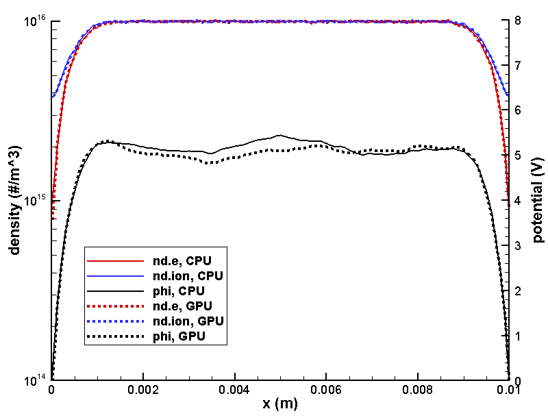
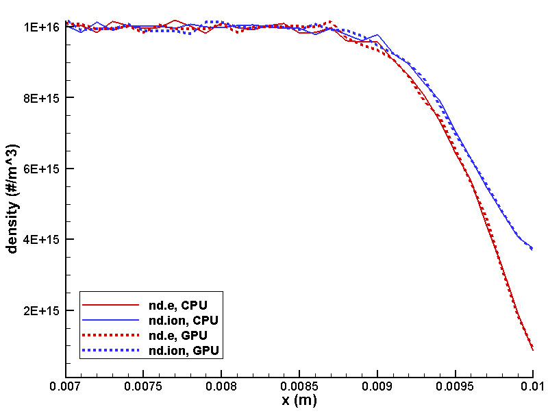
It took me about 2 hours to make the above changes and debug the code. So how did the code do? First, let’s take a look at results. After all, it doesn’t make sense to talk about performance if the results don’t agree. Figure 1 below plots ions and electron density, and potential from the CPU and GPU version using total of 1 million particles and 10,000 time steps. The results are very similar. The small difference in potential is expected. In these types of fully kinetic sheath simulations, potential oscillates quite a bit from time step to time step. This is due to statistical noise as ndi and nde are not exactly equal even in the neutral bulk plasma region due to a finite number of simulation macroparticles. The second picture shows a close up of the right wall, showing the density profiles follow each other.
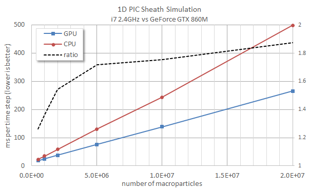
What about timing results? After all, all this work was done to hopefully gain some performance. Figure 2 shows results obtained on my laptop, which is a fairly standard system with an Intel i7 2.4GHz CPU and one GeForce GTX860M GPU. Both versions were launched through Visual Studio under “Release” mode so standard compiler optimization was applied. The left axis shows time (in milliseconds) per time step. Lower is better. Since only the particle push was moved to the GPU, we may expect the performance gain to improve as more particles are added. This is in fact the case. With half-million particles, the GPU version runs about 26% faster than the CPU code. As we increase the particle count to 20 million, the GPU version becomes 1.87 times faster. Quite far from an order of magnitude gain, but not a bad improvement for two hours of effort!
Future Work
Just to conclude, there is much effort that could be put in this code both on the CPU and GPU side to improve performance. Besides investigating memory access and different algorithms to avoid atomics, we could also take advantage of multi-threading on the CPU side. Specifically, we currently have two species that need to be pushed. While the GPU is doing this, the CPU is sitting idly. Instead, we could farm out only of the species to the GPU, and have the CPU perform computations on the other. This would yield the additional benefit of having one less cudaMemcpy as one of the species densities would already be stored on the CPU. All of these techniques will be discussed in more detail in the Distribute Computing course. Register to learn more.
Source Code
CPU version: sheath-cpu.cpp
GPU version: sheath-gpu.cu