The Finite Volume Method

The Finite Difference Method for solving differential equations is simple to understand and implement. However, it has one significant drawback: it can only be applied to meshes in which the cell faces are lined up with the coordinate axes. As such, it becomes difficult, if not out outright impossible, to resolve curved boundaries – like those encountered when dealing with any realistic geometry.
The Finite Volume Method (FVM) offers an alternative approach for deriving the discretized equations. This method is based on the principle that the divergence term, that frequently occurs in differential equations governing various interesting scientific phenomena, can be rewritten as a surface integral using the divergence theorem. The problem then simplifies to evaluating fluxes normal to the cell walls. Since this becomes a vector problem, the cell walls can take any shape and can be arbitrarily oriented. All that is required is that the they enclose a closed volume. And since the method is based on evaluating fluxes, the Finite Volume Method is conservative. Outflow from one cell becomes inflow into another. This makes the FVM stable and flexible, and yet relatively easy to implement. This is why the Finite Volume Method is commonly implemented in commercial computational fluid dynamics (CFD) solvers.
The Finite Volume Method
Consider the general Poisson equation, the governing equation in electrostatics, but also in other areas such as gas diffusion: \(\nabla^2\phi=b\)
In electrostatics, the right hand side is the negative charge density divided by the electrical permitivity. In diffusion, it becomes the species production rate. We can write this equation in the integral form by integrating both sides over some control volume. We then get
$$ \displaystyle \int_V \nabla \cdot \nabla \phi dV =\int_V b dV$$
or by employing the Divergence Theorem and assuming the value of the right hand side is constant over the control volume
$$\displaystyle \oint_S \nabla \phi \cdot \hat{n}dA =\tilde{b} \Delta V$$
where \(\Delta V\) is the volume of the control volume. Finally, we can approximate the integral on the left hand side by summing over the faces of our control volume. Assuming our control volume is a three dimensional Cartesian brick, we obtain (Eq. 1)
$$\displaystyle \sum_{i=1}^{6} \left(\nabla \phi\right)_i \cdot \left(\hat{n}dA\right)_i =\tilde{b} \Delta x \Delta y \Delta z \qquad\text{(1)}$$
Example
As an example, let’s consider the potential between two conducting cylinders shown in Figure 1. The domain of interest is the empty space with an annular geometry. This problem is both simpler and more complicated than the case presented in Eq. 1. It is simpler because if we assume the problem is axi-symmetric (quite a valid assumption), the problem becomes two dimensional. But it is more complex however since we are now dealing with the cylindrical coordinate system. But this coordinate system will allow us to better illustrate some of the details of FVM. For now, for simplicity, we will keep the computational mesh rectilinear. We will consider a more general case with arbitrarily shaped cells in a future article.
Potential is governed by the Poisson equation, \(\nabla^2\phi = -\rho/\epsilon_0\) which in cylindrical coordinates is (Eq. 2)
$$\dfrac{\partial^2 \phi}{\partial r^2} + \dfrac{1}{r}\dfrac{\partial \phi}{\partial r} + \dfrac{1}{r^2}\dfrac{\partial^2\phi}{\partial \theta^2}+\dfrac{\partial^2 \phi}{\partial z^2} = -\dfrac{\rho}{\epsilon_0}\qquad\text{(2)}$$
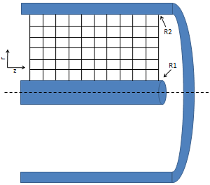
Figure 1. Domain is given by the annular region between two concentric cylinders.
Since the problem is axi-symmetric \(\partial \phi/\partial \theta=0\), the third term on the left vanishes. Also since the mesh is rectangular, we can easily obtain the discretized form using the finite difference method,
$$\displaystyle \frac{1}{r_{i,j}} \frac{\phi_{i,j+1}-\phi_{i,j-1}}{2\Delta r}+\frac{\phi_{i,j-1}-2\phi_{i,j}+\phi_{i,j+1}}{\Delta^2 r} + \frac{\phi_{i-1,j}-2\phi_{i,j}+\phi_{i+1,j}}{\Delta^2 z} = -\frac{\rho_{i,j}}{\epsilon_0}$$
Finite Volume Method in Cylindrical Coordinates
Of course, that is not what this article is about. As shown in Figure 2, we can draw a control volume around each grid node. Boundaries of this control volume are computed by joining centroids of the surrounding cells. Next we integrate the governing equation over this volume,
$$\displaystyle \int_V \nabla\cdot\nabla\phi dV=\dfrac{1}{\epsilon_0}\int_V\rho dV$$
For simplicity, the charge density on the right side is replaced by an average value, corresponding to the charge density at the grid node. The right hand side can then be integrated
$$\displaystyle \int_V \nabla\cdot\nabla\phi dV\approx\dfrac{\tilde{\rho}}{\epsilon_0}\Delta V=\dfrac{\tilde{\rho}}{\epsilon_0}r\Delta z \Delta r\Delta \theta$$
The right hand side is the approximation of the volume. In cylindrical coordinates, the three lengths are given by dr, dz, and rΔθ, respectively. This is shown in Figure 3. We next rewrite the integral on the left hand side using the Divergence theorem $$\int_V \nabla\cdot \vec{f}dV=\oint_S\vec{f}\cdot\hat{n}dA$$ and obtain integral form of our governing equation, $$\displaystyle \oint_S \nabla\phi\cdot\hat{n}dA=\dfrac{\tilde{\rho}}{\epsilon_0}r\Delta z \Delta r\Delta \theta$$

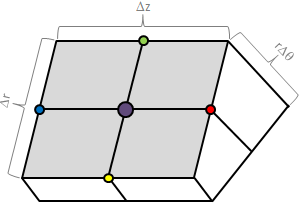
Figure 2. Two and three dimensional representation of the control volume. The central node is highlighted in purple.
Summation over Control Volume Faces
The surface integral can be evaluated by performing the summation over the four faces of the control volume, \(\displaystyle \oint_S \nabla\phi\cdot\hat{n}dA \approx \sum_{i=1}^4 \nabla\phi_i\cdot\hat{n}_idA_i \). Figure 2 should help you visualize this. We are summing over the two “white” faces, plus the other two corresponding hidden faces.
We evaluate the sum by going counterclockwise around the boundary, starting with the edge “1” (the red circle). At each face we dot the gradient with the normal vector multiplied by the face area. We need to take into account the rΔθ since this is the “thickness” (the part going into the monitor in Figure 2). Here r is the radius at the face centroid (the red, green, blue, and yellow markers). Due to our simple grid geometry, one of the two vector components vanishes, and we obtain the following expressions: \(\displaystyle \left.\frac{\partial\phi}{\partial z}\right|_1r\Delta r\Delta \theta\), \(\displaystyle \left.\frac{\partial\phi}{\partial r}\right|_2(r+0.5\Delta r)\Delta z\Delta \theta\), \(\displaystyle -\left.\frac{\partial\phi}{\partial z}\right|_3r\Delta r\Delta \theta\), and \(\displaystyle -\left.\frac{\partial\phi}{\partial r}\right|_4(r-0.5\Delta r)\Delta z\Delta \theta\), respectively.
After substituting and eliminating \(\Delta\theta\) from both sides we obtain
$$\displaystyle \left(\left.\frac{\partial \phi}{\partial z}\right|_1-\left.\frac{\partial \phi}{\partial z}\right|_3\right)r\Delta r +
\left(\left.\frac{\partial \phi}{\partial r}\right|_2-\left.\frac{\partial \phi}{\partial r}\right|_4\right)r\Delta z +
\left(\left.\frac{\partial \phi}{\partial r}\right|_2+\left.\frac{\partial \phi}{\partial r}\right|_4\right)0.5\Delta r \Delta z = – \frac{\rho}{\epsilon_0}r\Delta z \Delta r $$
and after dividing by the remaining volume components from the RHS, we obtain (Eq. 3)
$$\displaystyle \left(\left.\frac{\partial \phi}{\partial z}\right|_1-\left.\frac{\partial \phi}{\partial z}\right|_3\right) \frac{1}{\Delta z} +
\left(\left.\frac{\partial \phi}{\partial r}\right|_2-\left.\frac{\partial \phi}{\partial r}\right|_4\right)\frac{1}{\Delta r} +
\left(\left.\frac{\partial \phi}{\partial r}\right|_2+\left.\frac{\partial \phi}{\partial r}\right|_4\right)\frac{1}{2r} = – \frac{\rho}{\epsilon_0}$$
Note that this is nothing else but the definition of divergence in cylindrical coordinates. Pretty nifty!
Gradient Expression
Of course, we are not done yet. In order to evaluate Eq. 3, we need expressions for the four gradients. In the finite difference method these are easily obtained from the Taylor expansion. However, in order to illustrate the FVM method, and it’s application to generalized cell geometries, we derive the gradients again by considering a control “volume” around each of the four locations (the 4 colored circles in Figure 2) at which we require the gradients. However, the dimensionality of our problem has reduced, since we are now evaluating \(\int \nabla\cdot\phi dA\). What used to be volume integrals become surface integrals, and surface integrals become line integrals.
Figure 3 depicts the situation at the “red” node (location 1). We write an expression for the gradient using the scalar form of the divergence theorem, \(\displaystyle\int_A\nabla\phi dA=\oint_C\phi\hat{n}dl\). Taking the divergence as constant over the control area, we obtain \(\displaystyle\nabla \phi \Delta r\Delta z = \oint_C\phi\hat{n}dl \approx \sum_{i=a}^d\phi_i\hat{n}_idl_i \)

Figure 3. Control area used to compute gradient at face 1 (depicted by red node in Figure 2).
We next go around the control surface counter-clockwise and obtain the following
$$\nabla\phi_1 \Delta r \Delta z = \phi_a \Delta r \hat{e}_z + \phi_b \Delta z \hat{e}_r -\phi_c \Delta r \hat{e}_z -\phi_d \Delta z \hat{e}_r$$
Note that the rΔθ no longer appears here since we are integrating only over the gray face in Figure 2.
There is one issue here. While the locations a and c correspond to actual grid nodes, locations b and d do not. We need to approximate these. One option is to calculate these by interpolating data from neighboring grid nodes. And since these nodes are the cell centroids, their value is simply the average of the surrounding four nodes. This is where good node labeling comes in handy. While in your code you will use i and j grid indices, here we use the capital letters as shown in Figure 3 to correspond to the different nodes. We write \(\phi_a=F\), \(\phi_c=E\), \(\phi_b=0.25(E+F+H+I)\), and \(\phi_d=0.25(B+C+E+F)\).
Substituting we obtain
$$\nabla\phi_1 \Delta r \Delta z = \hat{e}_z\left(F -E\right) \Delta r +
\hat{e}_r[0.25(E+F+H+I-B-C-E-F)\Delta z$$
After a bit of elimination and we obtain
$$\nabla\phi_1 \Delta r \Delta z = \hat{e}_z\left(F -E\right) \Delta r +
\hat{e}_r[0.25(H+I-B-C)\Delta z$$
But look, in Equation 3 we only need the z component. We thus write
$$\displaystyle\left.\frac{\partial \phi} {\partial z} \right|_1 = \frac{F-E}{\Delta z}\equiv
\frac{\phi_{i+1,j}-\phi_{i,j}}{\Delta z}
$$
Similarly, we obtain
$$\displaystyle\left.\frac{\partial \phi} {\partial r} \right|_2 = \frac{H-E}{\Delta r} \equiv
\frac{\phi_{i,j+1}-\phi_{i,j}}{\Delta r}$$
$$\displaystyle\left.\frac{\partial \phi} {\partial z} \right|_3 = \frac{E-D}{\Delta z}\equiv
\frac{\phi_{i,j}-\phi_{i-1,j}}{\Delta z}$$
and
$$\displaystyle\left.\frac{\partial \phi} {\partial r} \right|_4 = \frac{E-B}{\Delta r} \equiv
\frac{\phi_{i,j}-\phi_{i,j-1}}{\Delta r}$$
These are the same derivative you would obtain (in much less effort!) with the finite difference technique. Of course, this FVM approach is more general since it can be applied to any shape cells.
Putting it all together
All that is needed now is to substitute these four expressions in Eq. 3. We obtain
$$\displaystyle \left(\frac{\phi_{i+1,j}-\phi_{i,j}}{\Delta z} – \frac{\phi_{i,j}-\phi_{i-1,j}}{\Delta z}\right) \frac{1}{\Delta z} +
\left(\frac{\phi_{i,j+1}-\phi_{i,j}}{\Delta r} – \frac{\phi_{i,j}-\phi_{i,j-1}}{\Delta r}\right)\frac{1}{\Delta r} +\left(\frac{\phi_{i,j+1}-\phi_{i,j}}{\Delta r} + \frac{\phi_{i,j}-\phi_{i,j-1}}{\Delta r}\right)\frac{1}{2r_{i,j}} = – \frac{\rho}{\epsilon_0}$$
or
$$\displaystyle \frac{\phi_{i+1,j}-2\phi_{i,j} + \phi_{i-1,j}}{\Delta^2 z} +
\frac{\phi_{i,j+1}-2\phi_{i,j}+\phi_{i,j-1}}{\Delta^2 r}
+ \frac{1}{r_{i,j}} \frac{\phi_{i,j+1}-\phi_{i,j-1}}{2 \Delta r} = – \frac{\rho}{\epsilon_0}$$
which is the same expression derived previously using the Finite Difference approach.
Verification
Just as with any numerical method, it is necessary to check our code to make sure the results are correct. This is the “verification” step of validation and verification (verification checks if the equations are being solved correctly, while validation checks if the equations themselves are correctly describing the problem).  If the right hand side forcing function is constant, potential is constant along each wall, and the slab is assumed to continue to infinity along the Z direction, then \(\partial \phi/\partial z=0\), and the problem becomes one dimensional. We can then analytically integrate \((1/r)(\partial/\partial r)(r\partial \phi/\partial r)=b\) to obtain
$$\displaystyle \phi=\frac{br^2}{4}+(\ln r)c_1+c_2$$
where
$$\displaystyle c_1=\frac{1}{\ln\frac{R2}{R1}}\left[\left(\phi_2-\phi_1\right)-\frac{b}{4}\left(R_2^2-R_1^2\right)\right]$$
and
$$\displaystyle c_2 = \phi_1-\frac{br_1^2}{4}-\frac{\ln R_1}{\ln \frac{R_2}{R_1}}\left[\left(\phi_2-\phi_1\right)-\frac{b}{4}\left(R_2^2-R_1^2\right)\right]$$
This analytical solution is plotted in the figure to the right using the solid black line for a case of fixed potential on both the inner and outer wall. We can next compare the numerical solution. It was “solved” using Excel. You can download the Excel Solver here. Feel free to play with the boundary conditions. Solution after 10 and 100 iterations is plotted in red. We can see that even though the numerical solution does not yet match the analytical solution after 100 iterations, the solution is indeed converging towards the expected profile.
References:
Anderson, D.A. and Tannehill, J.C. and Pletcher, R.H.,Computational fluid mechanics and heat transfer, 1984, Hemisphere Publishing, New York, NY
Here is a short paper on using multigrid to solve a similar type problem.
http://cd-amr.fnal.gov/aas/poisson.pdf
How would the Finite Volume Method compare with the multigrid method?
Here is my comparison of a multigrid solver versus gauss-seidel solver for solving this problem.
http://dl.dropbox.com/u/5095342/PIC/solverMg1D.html
The blue dashed lines are gauss-seidel solutions after 20, 40, 60 … 180 iterations, each time moving closer to the true solution. The red dashed lines multigrid solutions after 2, 4, 6, … 18 VCycles, also moving closer to the solution. The black dashed line is single Full Multigrid Cycle, which is very close to the true solution, after only one full multigrid cycle.
I downloaded your Excel sheet and I noticed that at each step, you used the phi[j+1] value of the previous step and also the phi[j-1] value of the previous step. Doesn’t phi[j+1], phi[j], and phi[j-1] all have to be taken at the same time? I thought they were only different spatially – phi[j+1] is on top of phi[j], which is on top of phi[j-1]. But when I tried to use all three values from the same time step, the values in Excel exploded to huge negative numbers. Any ideas? I appreciate your help and I love your site!!!
Hi Derek and thanks! The reason the code is blowing up when you use phi[j+1] from the current iteration is that this value is not yet known. Think of what happens the first time the code goes through. All nodes are initially set to some arbitrary initial value. The code then loops through the nodes starting with the first one. When you get to the jth node, the j-1 node has already been evaluated according to the governing equation, however, j+1 is still set to some arbitrary garbage value.
These iterative solvers basically work by marching the solution forward in a virtual time until “steady state” is achieved. This steady state is marked by the nodes no longer changing value, or at least changing so little that it’s within the prescribed tolerance. Hence it generally doesn’t matter if you use j-1 and j+1 from the previous iteration time (Jacobi method), or if j-1 is from the current and j+1 from the previous (Gauss-Seidel method). There are some exceptions as some equations will only converge with one approach and not the other, but this usually doesn’t happen with the sorts of equations you will normally encounter. The difference between the Jacobi and the GS approach is the convergence time, GS usually converges faster. But the solution will be the same.
There is an alternative way of solving differential equations, and that is with an implicit formulation, in which all values are taken at the current iteration time step. This is basically what you tried to do. However, this requires that all nodes are evaluated concurrently, since they all depend on each other. This in other words becomes a matrix inversion problem. The iterative methods are simpler to implement and also have a smaller memory requirement than these direct, implicit methods, and hence are used much more frequently. However, to get a flavor of how this works, you can see the article on particle integration in magnetic field, it has some examples of implicit methods.
Your website is very nice. In regards to the example on this page, I am confused about some of the values and how to obtain the value of phi/eps0. Do we have: 1) The inner cylinder is at 5V, 2) The outer cylinder is at 0V, 3) The radius of the inner cylinder is 0.1, 4) The radius to the inner surface of the outer cylinder is 0.2. Please reply at your convenience. Thank you kindly.
Hi Steve,
Those are the boundary conditions. You are solving an elliptic equation, in this case [latex]\nabla^2\phi=-\rho/\varepsilon_0[/latex], subject to these boundary conditions. The method shown on this page, the Finite Volume Method, is one procedure that allows you to obtain the values of phi inside the domain such that both the boundary conditions and the governing equation are satisfied.
Since all nodes depend on each other (the gradient is basically a weighted average, except with the central node having the opposite sign), you cannot directly calculate phi at every node. Instead, you have to keep iterating through the nodes. At each iteration you compute a correction to the node value. You repeat this until the governing equation is satisfied everywhere in the domain.
Hopefully this helps!
The equation you provide in you Example section for the finite difference equation is not quite right. The second and third term have the pattern 1 -1 1 instead of 1 -2 1 . The “Putting it all together” section gets the equation right but doesn’t match your “previously derived” equation from the Example section in the article.
Hi John, which equation are you talking about? You can use the latex syntax if you want, just enclose it in latex and /latex in square brackets.
I am not familiar with latex syntax and I tried cutting and pasting the equation from the blog post into this comment but it did not show up.
Anyway, if you can’t see the equation between the latex tags above, then the equation I am refering to is the one at the end of the section entitled “Example” in this blog post, just below the words “the finite difference method”.
The term -1*phi(i,j) in this equation should be -2*phi(i,j) for a second difference equation.
The equation at the end of the “Putting it all together” section of the blog gets it right.
Ok, I see it. I corrected it above. Thanks for the tip!
Just below the figure 3, last 2 terms in the equation, I guess vectors are written wrong. They should be -() e_z – (e_r).
Thanks Dinesh, I have corrected the subscripts.
Lubos, I need more detail about this method for implementing diffusive term by calculating gradient on faces. Can you please tell me some reference book, code available or algorithm using similar method. Would be better if I could see this implementation in a 2D code available. As most of the book or notes they calculate N,E,W,S method.
Thanks
In your FVM blog post you mentioned “We will consider a more general case with arbitrarily shaped cells in a future article.”. Do you have any plans on creating a FVM blog post for arbitrary shaped cells in the near future? I have come across some MATLAB code for generating a mesh for an arbitrary shaped 3D object and would like to know how to solve the poisson equation using FVM on the mesh nodes and tetrahedra.
http://persson.berkeley.edu/distmesh/
Also, do you think that the FVM is preferrable to the Finite Element Method when working with plasma simulation solvers?
Heh, I do, just can’t find the time 🙂 But it will be coming very soon (I am basically trying to balance blogging and actually getting work done but it’s not all that easy…)
And thanks for the Distmesh link. I’ve used it in the past but forgot about it. It’s a very neat tool.
OK, looking forward to it. By the way, I had to make a few small changes to distmesh to get it to work with Octave. Octave complained about a few things but they were easy to fix. I am able to run meshdemo2d and meshdemond commands in Octave to produce 2D and 3D meshes of the objects included in these demos. You will likely encounter the same problems I did if you try distmesh with Octave. I reported the problems to the author so hopefully he will update the code to fix the Octave issues.
This website is amazing. I have one question about axi-symmetric cylindrical coordinate using fintie difference method. How to present the first term 1/ri,j in the code? Could you please write a code in matlab by uisng the fintie difference method to solve the axis-symmetric cylindrical coordinate? I am really appreciating for that!!!
Thanks Boyuan. I do plan to write a follow up article shortly demonstrating the use of this method on some non-rectangular domains. Is your question about r at r=0? This is the axis of symmetry, and hence you require $latex \nabla \phi = 0$ here (i.e no kinks). This Neumann boundary condition will eliminate the need for r.
hi. a solid explanation of the FVM, thanks. one question remained to me after reading the text for the first time. the method solves the poisson equation in a given volume. boundary values of phi are given (at least i think so). while operating, the code “fills” the grid postions with the a priori unknown phi values. isnt there a problem in the “Gradient Expression” section, if the values phi_a,..,phi_d arent known a priori?
Hi Alex, I am not sure I follow. Are you talking about the boundary values? You can have different types of boundaries, such as Dirichlet (prescribed potential) or Neumann (prescribed potential gradient). You may need to adjust the expressions along the boundaries. But internally, the scheme works in an iterative fashion. Each pass gets you closer to the solution (at least in theory, assuming it is converging). You continue iterating until the error given by the norm of the residue reduces to some small value.
I have spent an hour trying to figure out what is going on in the section titled “Gradient Expression”, and only now beginning to understand why it was so difficult to understand. I think it would be helpful if you used a vector-del notation rather than just del. This allows readers to know what things are vectors and what are scalars.
i want to write matlab code for finite volume method in implicit method please help
Hey, I would like to solve the electric field equation for multiple cylinders in a single cylindrical geometry, like many inner cylinders (likely 4) within one huge cylinder. How to proceed on?