Nonlinear Poisson Solver

One of the governing equations for electrostatic plasma simulations is the Poisson’s equation,
$$\nabla^2\phi=-\dfrac{\rho}{\epsilon_0}=-\dfrac{e}{\epsilon_0}\left(Z_in_i-n_e\right)$$
In the types of discharges we typically consider here at PIC-C, the ion density is obtained from kinetic particles (the particle-in-cell method) while electrons are approximated as a fluid. The electron thermal velocity assuming 5eV electrons is over one million meters per second. On the other hand, typical ion velocities in plumes are around 15 km/s. This is a speed ratio of three orders of magnitude. The PIC method requires that particles travel less than a cell length per time step. As such, the simulation time step will be determined by the fastest species. Hence, if want to include electrons, we need to run the simulation at 1000 times smaller time step than what would be satisfactory for the ions. In other words, the simulation will take 1000 times longer to complete the same physical time span.

Boltzmann relationship

Luckily, we can often get away with not simulating electrons as kinetic particles. This is true especially when magnetic fields are not present or we are dealing with motion in direction along the magnetic field lines. Consider the electron momentum equation,
$$mn\left[\dfrac{\partial \mathbf{v}}{\partial t} + \left(\mathbf{v}\cdot \nabla\right)\mathbf{v}\right]=qn\mathbf{E}-\nabla p$$

In the frame of reference of ions, electrons are seen to respond instantaneously to a disturbance, and thus the time dependent term can be neglected. The convective term can also be generally neglected since its magnitude is small (or zero if we consider spatially uniform velocity). This then leaves us with the force balance, \(q\mathbf{E} = \dfrac{1}{n}\nabla p\). We can next make three substitutions, \(q=-e\), \(\mathbf{E}=-\nabla \phi\), and \(p=nkT_e\) (assuming isothermal electrons), which gives us \(e\nabla\phi = \dfrac{kT_e}{n}\nabla n\). This equation can be easily integrated along some arbitrary path to obtain
\(e\left(\phi-\phi_0\right)=kT_e\ln\dfrac{n}{n_0}\). This very important relationship is known as the Boltzmann relationship. It is encountered frequently in plasma physics. The importance of the Boltzmann relationship lies in the fact that it relates local potential and the local electron density. Given a set of reference parameters, electron potential can be computed everywhere in the domain (where the governing assumptions hold) from simply knowing the electron density.

Nonlinear Poisson’s Equations

The Boltzmann relationship can also be inverted to obtain an expression for electron density,
\(n_e = n_0\exp\left(\dfrac{\phi-\phi_0}{kT_e}\right)\)
This is the missing piece needed for our electrostatic potential solver! Instead of simulating electrons as particles, we can use this relationship directly in the Poisson’s equation,
$$\nabla^2\phi = -\dfrac{e}{\epsilon_0}\left[Z_i n_i – n_0\exp\left(\dfrac{\phi-\phi_0}{kT_e}\right)\right]$$
Unfortunately, this relationship results in a non-linear equation, since now the expression we are solving for (potential) appears on the right hand side as well. In matrix form, we have \(\mathbf{A}\phi=f(\phi)\). Luckily, solving non-linear equations is no rocket science – we just need little help from Mr. Newton.

Newton’s Method for Systems

Newton’s method is a simple algorithm for finding function roots. Consider some arbitrary equation \(f(x)=0\). We can use Taylor’s expansion to compute the value of this function in the vicinity of a known point, \(f(x)=f(\bar{x}) + (x-\bar{x})f'(\bar{x}) + O(2)\). For small differences the second order terms drop out and we can write
$$f(x)=0\approx \bar{x}-\dfrac{f(\bar{x})}{f'(x)}$$

Numerically, the above equation is used to get consecutively closer approximations to the function root, x_new = x_old - f(x_old)/f_prime(x_old). We can use a similar approach to treat a system of equations. The matrix analogue to the single equation is \(\mathbf{x}^{k+1} = \mathbf{x}^{k} – \mathbf{J}^{-1} \mathbf{F(x}^{k}\mathbf{)}\), where
$$
\mathbf{J}(x) = \dfrac{\partial f_i}{\partial x_j}(\mathbf{x}) = \left[\begin{array}{ccc} \dfrac{\partial f_1}{\partial x_1}(\mathbf{x}) & \dfrac{\partial f_1}{\partial x_2}(\mathbf{x}) & \ldots \\[0.3cm] \dfrac{\partial f_2}{\partial x_1}(\mathbf{x}) & \dfrac{\partial f_2}{\partial x_2}(\mathbf{x}) & \ldots \\[0.3cm] \vdots & \vdots & \ddots \end{array}\right]
$$
is the Jacobian. This algorithm is generally implemented in two steps two avoid the need to compute a matrix inverse. First, the \(\mathbf{J}(\mathbf{x})\mathbf{y}=\mathbf{F}(x)\) system is solved for \(\mathbf{y}\) using your favorite linear solver. The solution is then updated as \(\mathbf{x}^{k+1}=\mathbf{x}^{k}-\mathbf{y}\). The process continues until \(||y||<\epsilon_{tol}\), some prescribed tolerance.

The non-linear Poisson solver algorithm

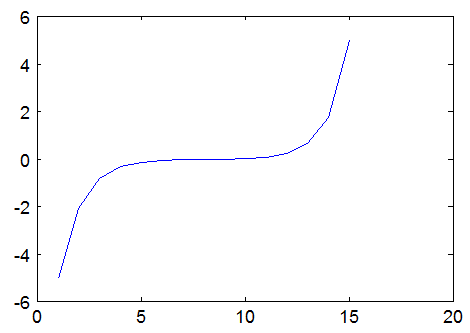
So how does this method look in practice when applied to the Poisson’s equation? Scroll down for the entire Matlab source code (note, the coding was actually done in Octave since we don’t have access to a Matlab license). To keep things simple, we apply the algorithm to a 1D system bounded on both ends with fixed potential nodes. The potential is -5V on the left boundary and +5V on the right boundary. Uniform plasma density of \(n_0=10^{16}\; \text{m}^{-3}\) and temperature \(kT_e=5\;\text{eV}\) is used.

Using the standard finite difference algorithm, we can write our governing equations as
$$\begin{array}{rcl}\phi_1&=&-5\\\phi_1-2\phi_2+\phi_3&=&Cn_{i,2} – C n_0\exp[(\phi_2-\phi_0)/kT_e]\\
\phi_2-2\phi_3+\phi_4&=&Cn_{i,3} – C n_0\exp[(\phi_3-\phi_0)/kT_e]\\
\vdots & = & \vdots\\
\phi_{n} &=& 5
\end{array}$$
Here the constant \(C=-e/\epsilon_0 \Delta^2h\). In other words, we have the system \(\mathbf{A}\mathbf{x} = \mathbf{b_0} + \mathbf{b_x}(\mathbf{x})\) (we are using \(\phi\equiv x\) for generality). The two vectors on the right hand side correspond to the constant and the non-linear term. As the first step in our algorithm, we compute the non-linear vector (the linear doesn’t change between iterations).

%1) compute bx
for n=1:nn
    if (fixed_node(n))
        bx(n)=0;
    else
        bx(n) = -C*den0*exp((x(n)-phi0)/kTe);
    end
end

The example is made more general by using a fixed_node array to indicate which nodes are fixed and which are fluid. We compute electron density only on the fluid nodes. Next we add the two right hand side vectors and subtract to obtain \(\mathbf{F(x)} = \mathbf{A}\mathbf{x} – \mathbf{b} = 0\).

%2) b=b0+bx
b = b0 + bx;
 
%3) F=Ax-b
F = A*x-b;

We next need to compute the Jacobian. Our function \(\mathbf{F(x)} = \mathbf{A}\mathbf{x} – \mathbf{b_0} – \mathbf{b_x}\) consists of three terms: the linear system given by the matrix multiplication, a vector which is not a function of x, and another vector which is. The derivative of the non-linear RHS vector is \(\partial (b_x)_i/\partial x_j = -\delta_{i,j}Cn_0\exp[(\phi_i-\phi_0)/kT_e]/kT_e\). The Jacobian is thus given by \(\mathbf{J}=\mathbf{A}-\partial (b_x)_i/\partial x_j=\mathbf{A}-\text{diag}(\mathbf{P})\). We first compute this P vector on fluid nodes,

%4) compute P=dbx(i)/dx(j), used in computing J
for n=1:nn
    if (fixed_node(n))
        P(n)=0;
    else
        P(n) = -C*den0*exp((x(n)-phi0)/kTe)/kTe;
    end
end

and set the Jacobian,

%5) J=df(i)/dx(j), J=A-diag(dbx(i)/dx(j))
J = A - diag(P);

The rest is easy. We first solve for y and then use it to update the solution. The final profile is plotted in Figure 1.

%6) Solve Jy=F
y = J\F;
 
%7) update x
x = x - y;

The iterations continue until convergence

%8) compute norm;
l2 = norm(y);
if (l2<1e-6)
    disp(sprintf("Converged in %d iterations with norm %g\n",it,l2));	
    break;
end

Complete Source Listing

Here is the complete source code in Matlab. The code was actually tested using Octave, so let us know if it doesn’t work in Matlab proper. Also, feel free to contact us if you need a Java implementation.

%Demo non-linear Poisson solver
% we are solving:
% d^2phi/(dh^2) = -rho/eps0*(ni-n0*exp((phi-phi0)/kTe))
% with phi=-5, 5 on left and right boundary
% See https://www.particleincell.com/2012/nonlinear-poisson-solver/ 
% for additional info
 
%clear screen
clc
 
%constants
EPS0 = 8.85418782e-12;	
Q = 1.60217646e-19;
 
%setup coefficients
den0=1e16;
phi0=0;
kTe=5;
 
%precomputed values
lambda_D = sqrt(EPS0*kTe/(den0*Q));	%for kTe  in eV
dh = lambda_D;				%cell spacing
C = -Q/EPS0*dh*dh;
 
%setup matrixes
nn=15;			%number of nodes
A=zeros(nn,nn);
fixed_node = zeros(nn,1);
b0=zeros(nn,1);
 
%left boundary
A(1,1)=1;
b0(1)=-5;
fixed_node(1)=1;
 
%right boundary
A(nn,nn)=1;
b0(nn)=5;
fixed_node(nn)=1;
 
%internal nodes
for n=2:nn-1
	%FD stencil
	A(n,n-1)=1;
	A(n,n)=-2;
	A(n,n+1)=1;
 
	fixed_node(n)=false;
	b0(n)=C*den0;
end
 
%initial values
bx = zeros(nn,1);
P = zeros(nn,1);
J = zeros(nn,nn);
x = zeros(nn,1);
y = zeros(nn,1);
 
%--- Newton Solver ----
for it=1:20
 
	%1) compute bx
	for n=1:nn
		if (fixed_node(n))
			bx(n)=0;
		else
			bx(n) = -C*den0*exp((x(n)-phi0)/kTe);
		end
	end
 
	%2) b=b0+bx
	b = b0 + bx;
 
	%3) F=Ax-b
	F = A*x-b;
 
	%4) compute P=dbx(i)/dx(j), used in computing J
	for n=1:nn
		if (fixed_node(n))
			P(n)=0;
		else
			P(n) = -C*den0*exp((x(n)-phi0)/kTe)/kTe;
		end
	end
 
	%5) J=df(i)/dx(j), J=A-diag(dbx(i)/dx(j))
	J = A - diag(P);
 
	%6) Solve Jy=F
	y = J\F;
 
	%7) update x
	x = x - y;
 
	%8) compute norm;
	l2 = norm(y);
	if (l2<1e-6)
		disp(sprintf("Converged in %d iterations with norm %g\n",it,l2));	
		break;
	end
end
 
disp(x');
plot(x);

You may also be interested in the article on solving potential n composite dielectrics.