Advanced PIC Course Debrief

Perhaps you noticed that I haven’t posted in a while. In fact, the latest article prior to today was posted over 4 months ago. One of the reasons was the Advanced PIC course. I find teaching quite interesting, but at the same time, I majorly underestimated the amount of time required to get the material ready.
I got the idea to offer online introductory PIC course back in 2014, shortly after completing teaching an actual live course at the George Washington University. The PIC course was well received so I decided to offer it again in 2015. I also decided to offer a follow up Advanced PIC course. While the Intro course discussed only the electrostatic particle in cell (ES-PIC) method on structured meshes, the advanced course delved into topics such as electromagnetics, DSMC, and unstructured meshes. These were all topics that I had worked with at some points in the past, but are not exactly things I touch on a daily basis. Most of my plasma codes are electrostatic and formulated on structured meshes. In fact, lately I’ve been developing codes for modeling contamination and those don’t even need a mesh. In other words, this course was bit of a learning experience for me as well. I wanted to brush up on EM and FEM, and there is no better way than by teaching someone else. The downside is that it took me a while to get the examples and slides ready. In the end, instead of consisting of 8 lessons over 8 consecutive weeks, the course ended up being 11 lessons spanning over 3 months. The idea behind this post was to summarize the course, and to also put down some observations and hopefully get feedback to make improvements for 2016.
Lecture Summaries
Lecture 1
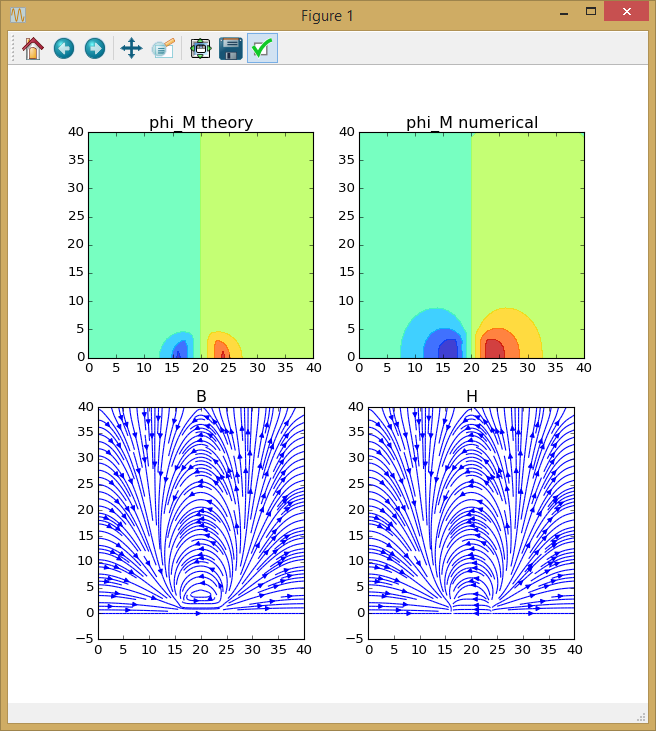
The class started with an overview of the PIC method. These overview slides came from the Fundamentals course so preparing this part of the lecture was not difficult. Next, we introduced a potential solver on dielectric materials. This mainly involved describing ideas from this article so this part also didn’t take long to prepare. We then moved into magnetostatics (Maxwell’s equations without a varying electric field). We developed a simple Python program to compute the magnetic field around a magnetized object using the scalar potential method. This result is shown in Figure 1.
Lecture 2
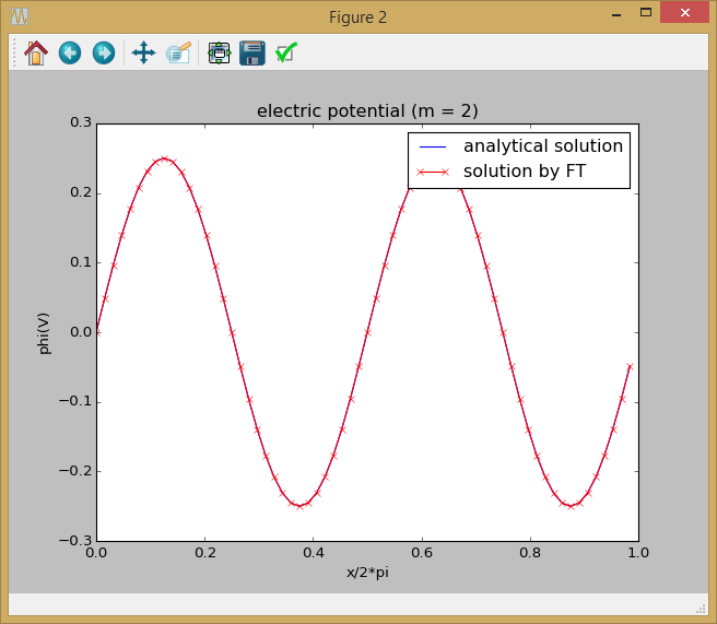
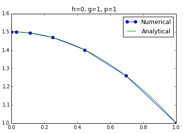
The next lecture started with a brief mathematical overview of waves. We then started developing equations for a 1D EM-PIC solver in CGS units, following the formulation in Birdsall. This allowed us to introduce the concept of advancing E and B fields. After the math overview, I introduced Discrete Fourier Transforms and using them to solve PDEs. For homework, the students were asked to write a DFT solver, with result shown in Figure 2.
Lecture 3
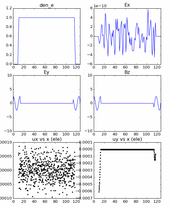
This lesson started with a continuation of the discussion on Fourier Transforms. We saw how to use them on non-periodic problems, by including a “vacuum moat”. We then developed the 1D EM-PIC code according to the equations from Lesson 3. Snapshot of the results is in Figure 3. This is actually a frame from an animation.
Lecture 4
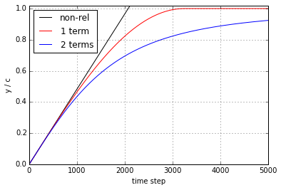
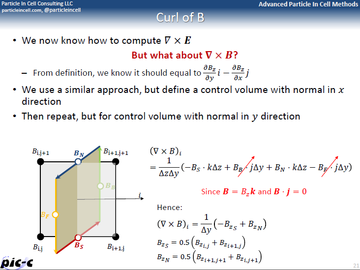
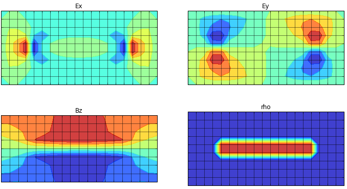
Lesson 4 started with a discussion of relativistic push. We compared results with a “one term” and “two term” scheme, with the “one term” form being quite common in EM-PIC codes. We then saw how to develop an EM-PIC code in 2D, following some papers of my Master’s adviser, Joe Wang. This involved describing a staggered mesh, and numerical schemes for computing divergence and curl. These codes were also developed in Python.
Lectures 5 and 5.5
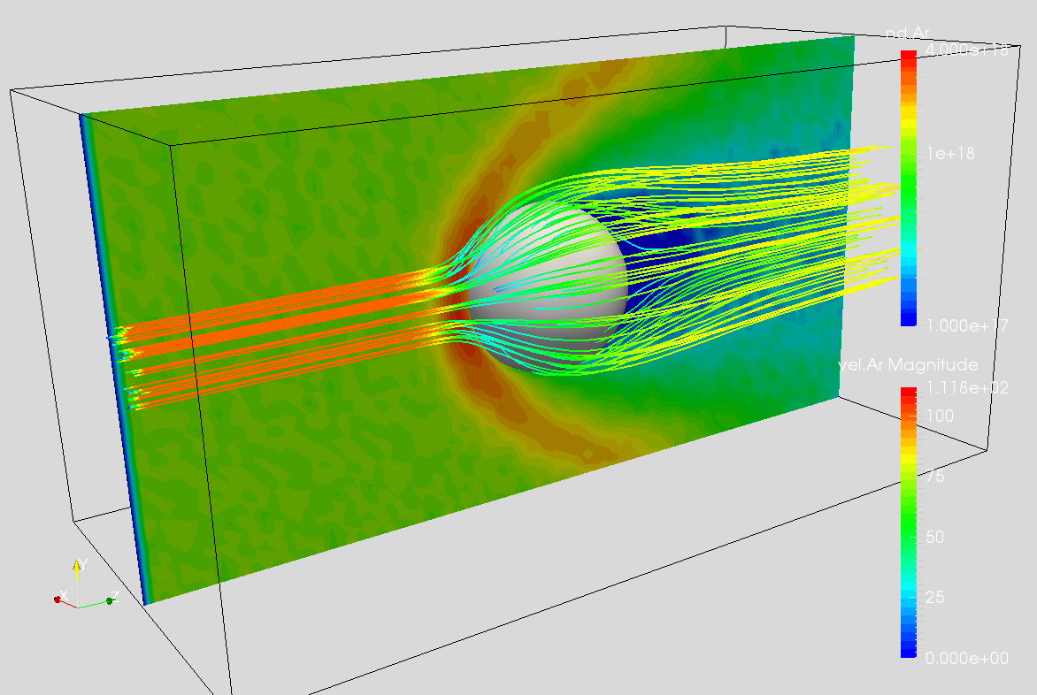
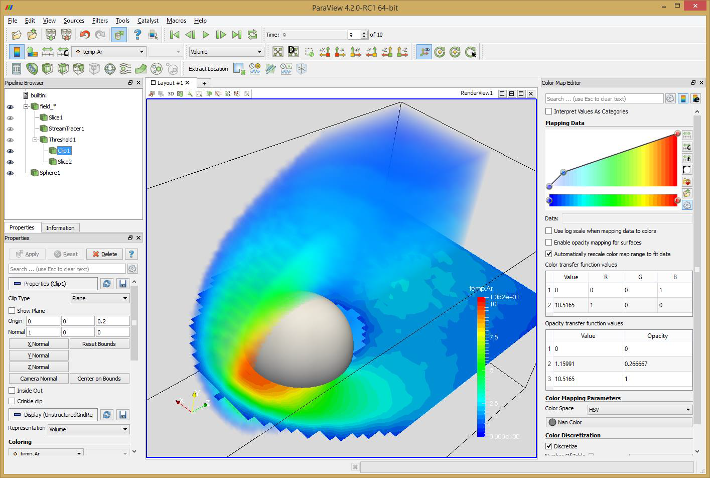
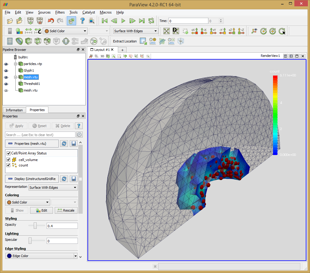
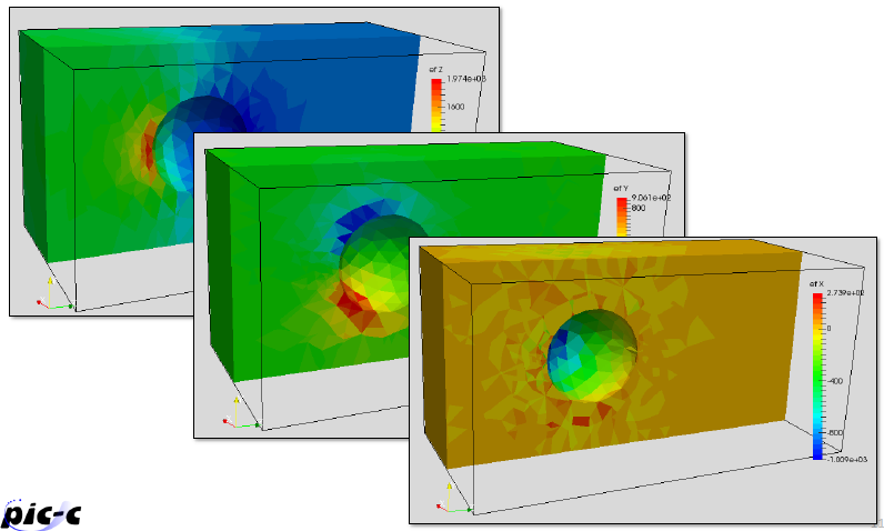
Lesson 5 was supposed to be a single lesson on modeling collisions. However, during the week of this lecture, we ended up relocating from Virginia to California, so between packing and driving cross country, there was not much time left to prepare the full lecture. So I held a short Lesson 5 which went over the math behind the DSMC method from Bird. The real lesson 5 was titled “Lesson 5.5” and was held two weeks later. We started this lecture by discussing particle shape factors. I then demonstrated difference between MCC and DSMC with a simple 1D example, which allowed us to talk about momentum (or the lack of) conservation. We then developed a 3D DSMC code to model the flow of neutral gas around a sphere. We also saw how to compute macroscopic parameters such as temperature from particle data. We used Paraview to visualize the results, as shown in Figure 5. In this lecture we also switched from Python to C++.
Lecture 6
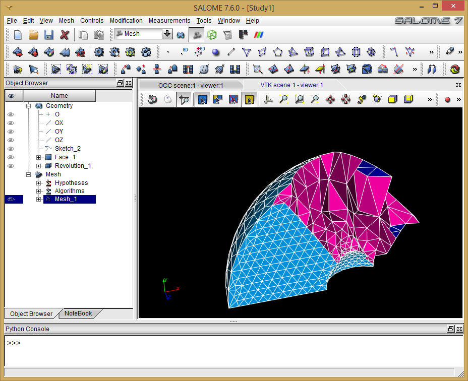
In lesson 6 we started taking the first steps towards a PIC code on an unstructured mesh. This first required learning how to move particles on an unstructured mesh, which then in turn required generating such a mesh. We started the lecture by learning how to use Salome to draw a simple part and create a tetrahedral mesh. We exported the mesh to a text file and wrote a mesh loader. Next we learned about moving particles on an unstructured mesh. This involved learning about shape factors on a tetrahedral mesh and determining if a particle is located in a cell.
Lecture 7
The particle push code written in Lesson 6 was very inefficient as it required looping over all elements for all particles. Here we learned how to speed up the code by using neighbor search, similar to what is outlined in the dissertation of Mark Santi. Next, we moved to a different topic originally planned for Lesson 5, and learned how to join particles using ideas from the dissertation of Justin Fox. We closed the lesson by starting a crash course on the Finite Element Method (FEM), following Hughes. We developed a 1D FEM solver with analytically computed stiffness matrix.
Lecture 8, 8.5, and 8.6
Lesson 8 again ended up being split over multiple lectures. This was partly due to me running behind in getting the material ready, and also underestimating how many slides will be needed to cover everything. The first lecture was a short class in which we learned how to build the stiffness matrix and the force vector automatically from element data. Homework asked students to write a 1D FEM code that build the linear system automatically.
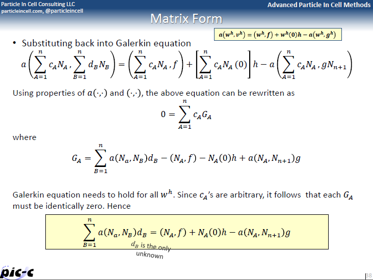
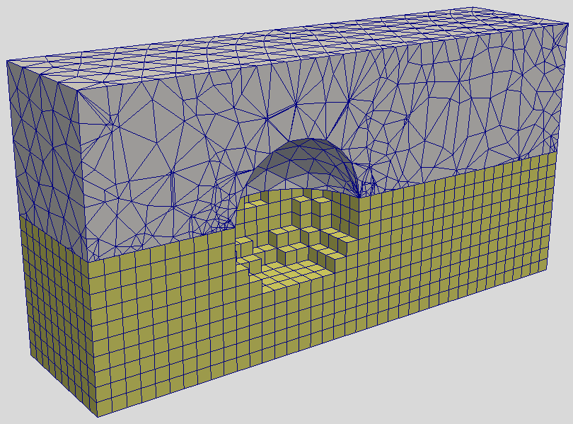
The next lecture was titled “Lesson 8.5”. In this lecture we used Salome to create a mesh for flow past a sphere. Since we needed the ability to flag the inlet and sphere nodes as Dirichlet boundaries, we also learned about mesh groups and modified the loader to support them. We then discussed the Galerkin equations in 3D, and learned about Gaussian quadrature and derivatives of shape functions. We concluded the lesson by developing an FEM solver for the linear Poisson’s equation.
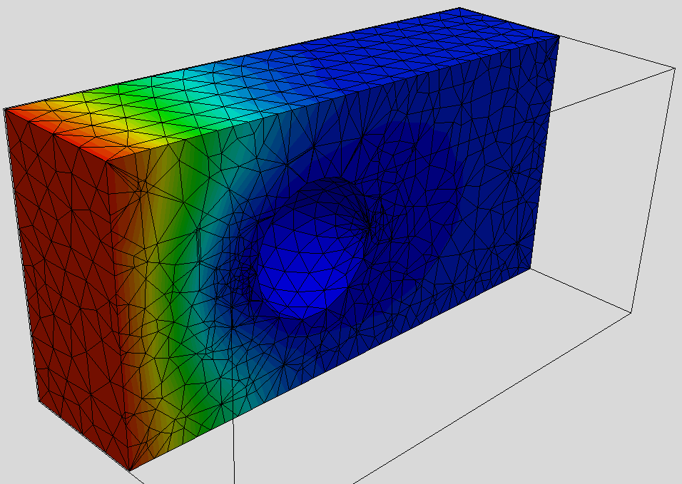
The above Lesson 8.5 concluded the course. But since we didn’t quite complete all that was on the syllabus, I put together one more set of slides (these went out about a month after Lesson 8.5) tying the loose ends. In the first part, we developed a finite element solver for the non-linear Poisson’s equation (non-linear due to the Boltzmann electron term) using the Newton-Rhapson method. We then combined the solver with the particle pusher from Lesson 7 to complete a 3D Finite Element Particle In Cell code.

Observations
One thing that surprised me about this course was that more people registered for it than for either of the two previous PIC fundamentals courses. The course had 14 students, while the PIC Fundamental courses averaged around 10. But, the participation wasn’t that great. Participation in the lectures dropped from about eight students the first two lectures to just one at the end. This was fine in the sense that the lectures were recorded and posted online, however, I was expecting more questions from students. This was also reflected in the homework. While 10 students completed homework 1 (an FFT solution), only one student completed all five assignments. To large extent, this is partly my fault due to a very erratic schedule of the lessons. At the same time, I suspect some of the material was bit too advanced for the students. There were also several students from whom I did not receive any emails nor have I seen them attend any of the lectures. I observed a similar thing the Fundamentals course. If any of the readers here have experience with teaching online courses, I would like to hear your takes on improving participation.
The second observation or more of a lesson learned is that I vastly underestimated the amount of effort required to get this course ready. It may seem strange, but what probably took the longest was putting together the PowerPoint slides. First, there was a lot of material to include, and secondly, PowerPoint doesn’t seem to like a lot of equations per slide as this often brought the program to a crawl. This resulted in me running late in getting the lessons ready which then ended up with us meeting at various erratic times, as opposed to a fixed schedule. This made it probably even more difficult for the students from outside the United States to attend the lectures, since some of the times were in the middle of the night for them.
Finally, in this course we used only two programming languages: Python and C++. In contrast, the Fundamentals course utilized four: Octave (Matlab emulator), Java, C++, and Python. I think reducing the number of languages helped. My original thinking was to allow students to see how the codes can be implemented in different languages, but I think that in the end it just led to confusion. The combination of Python and C++ works great, I think, as Python is suitable for introducing algorithm, but lacks the computational power of C++ needed for 3D programs.
Future
I plan to offer this course again in 2016. Since I now have all the examples and slides ready, the next version should go much smoother. Students signed up for the 2015 will be able to retake it for free, as I would like them all to complete the homework assignments and hence get the certificates. In addition, I will also offer the PIC Fundamentals course, and a new course on developing parallel PIC and fluid codes with multithreading, MPI, and CUDA. Stay tuned for more details.
Feedback
I would love to hear the feedback from you if you have taken the course. Feel free to leave a comment below – you can just put in some arbitrary values for the name and email field if you want it to be anonymous.
Dear Lubos
Are you planning to provide this course in India? Or by any means can it be accessed via net?
Ashish
Hi Ashish,
Yes. In fact, several students taking the course were from India. The course is conducted over GoToMeeting. The main difficulty is probably the time difference. We ended up moving the start time for the 2015 course to 5pm Pacific Time, which I believe is around 7am in India. I’ll most likely keep the same start time in 2016.
I have taught several free classes to consultants when a new technology came around. I always found a big drop off. Lately I have taken several Coursera courses and they have had huge attrition rates. It is probably due to people wanting to learn (easy part), signing up for the course (easy part) but don’t really have the time to dedicate to actually learning the material (hard part).
The PIC class that I took required a significant level of programming skill. This may have been a problem for some people.
You may want to add a forum for students to interact with you and other students.
Ken
Hi Ken,
Good idea on the forum. I’ll try to implement it. I am also wondering if having the lectures every two weeks instead of every week would be better as it would give students more time to catch up?
I very much enjoyed taking both the ES-PIC and EM-PIC courses. But the schedule was stretched a bit in Advanced Pic so i could not really complete the course. But i will go through most of the materials at my own pace. And yes sir, it would be nice to have a forum where students could interact.
I would like to give my feedback (more of an experience) on the course. It was really a great course. I had difficulties after first few weeks because of the complexity of the course. I had a lot of gaps in my knowledge. I clearly should have learned a few things ahead. Granted that i had never taken a formal course in plasma physics and only learned as things went by in ES-PIC. Advance PIC required a very good understanding and most of the lectures could have branched to form their own course too (DSMC, FVM … ). But i think that this may have not been a problem for a lot of people in the course. Duration was another bottleneck in the course. Since the course was a bit too stretched, it became a little difficult to multi task academic, personal and course activities. As someone mentioned above in the comments section, having a forum would be a really good thing. It would probably help all the students to at least engage with each other, share their background knowledge and keep in touch so that there is a continuity and a classroom feel to the course. It was really great that you used Python and C++. It really helped me understand what was going on exactly besides my lack of some of the subject knowledge. I notice you mentioned some of the shortcomings of python and one of them is Speed. I humbly request you to have a look at http://cython.org/ which is a really nifty way to get a C – Like speed in Python itself. It integrates well with numpy too. It also allows parallelization. This way you could eliminate even having two languages. You also mentioned the issues with powerpoint sir. I really think Latex Beamer would be much useful for you since you could practically re use the equations in your blog / manual / book if you are eventually interested in writing one. In every way possible, both the courses are nothing short of a gift to a student from a developing country like myself. It is really hard to find people who have a decent knowledge on the subject. Even if someone exist, they are not willing to spend any time at all in teaching a class to a person who isn’t their grad student. I read that you will be teaching a course on parallelization. I will most certainly be signing up for it too. I hope my feedback / experience is useful to you in some way sir.
Hi Vijai, thank you for your comments and for taking the classes! I will definitely try to implement the forum in some way. This will require redoing the student area, but that was something I was already planning on doing anyway. I also think that I should put together few pages on basics of object oriented programming and C++11 additions such as vectors, as I suspect some students are not very familiar with this. About cython, I’ll take a look, but I still think that for actual computational codes, you are better of developing them straight in C++. Or if you need GUI, then in Java. I actually very much like Java, but it seems that most people prefer Python or C++, hence my decision not to use Java in this course.
This course along with the course on fundamentals of PIC has been really helpful to me. I think, those who joins PhD in plasma physics and are willing to do some numerical work, should take this as their coursework in the beginning. The course content is quite detailed and has been developed in step by step. Moreover, there is a well maintained pace of learning. I too recommend a student forum and if possible then an open discussion on the ongoing research problems could be made.
Thanks Rakesh for your comment and taking the course!