Arduino Plasma Simulation

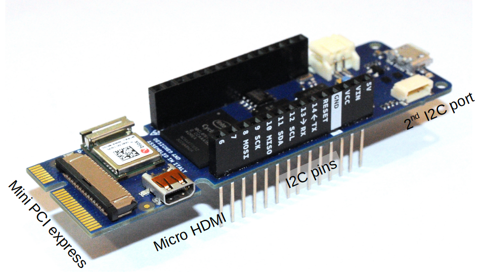
Those of you who have been following my LinkedIn page, the PIC-C Twitter account, or just saw the recent article on computing pi, have likely gathered that I have recently been spending much time “playing” with embedded programming, mainly using Arduino microcontrollers and Intel FPGAs. I am particularly excited about the relatively new Arduino MKR Vidor 4000 which comes with an integrated Intel Cyclone 10LP FPGA. My long-term goal is to use this (or a similar) system to put together a plasma simulation library that can be used to run analysis in parallel with hardware. Doing so would lead to many new “disruptive” technologies. For instance, we could simulate a plasma thruster while it is running to perform speculative predictions for operating conditions to maximize thrust or life time. Or space weather satellites could instead use such simulations to determine which data is of interest (perhaps not following classical models) to reduce the needed communication bandwidth.
Just as a proof of concept, I put together a simple PIC simulation (see the blog post or my book for more background) that can run on the Arduino. There is nothing specific about this code that limits it to the Vidor except that available memory may be smaller on one of the legacy boards. The simple code basically simulates a one-dimensional ion expansion. Ions are born at the left boundary, where \(\phi_{left}=0\). On the right boundary, potential varies sinusoidally,
$$\phi_{right}=-10\cos\left[2\pi\cdot\frac{ t_s}{200}\right]$$
here \(t_s\) is the current time step. Potential on the internal nodes is obtained from the non-linear Poisson’s equation,
$$\nabla^2\phi = \frac{e}{\epsilon_0} \left(n_i – n_0\exp\left[\frac{\phi-\phi_0}{kT_{e,0}}\right]\right)$$
We solve this equation with 100 iterations of the “poor-man’s” Gauss-Seidel. No convergence checking is done in this simple demo code. While one-dimensional Poisson’s equation can be solved much faster using the tridiagonal Thomas algorithm, that step would require a non-linear Newton-Raphson wrapper, and hence this GS approach was simpler to implement (even if slower). The code injects a fixed number of ions at each time step. The initial velocity is obtained by sampling from a uniform distribution, which is not quite right (should sample the Maxwellian), but again a little shortcut for the quick demo!
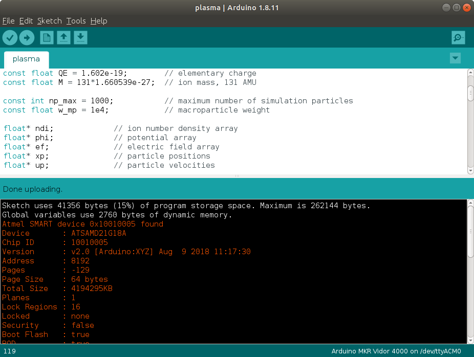
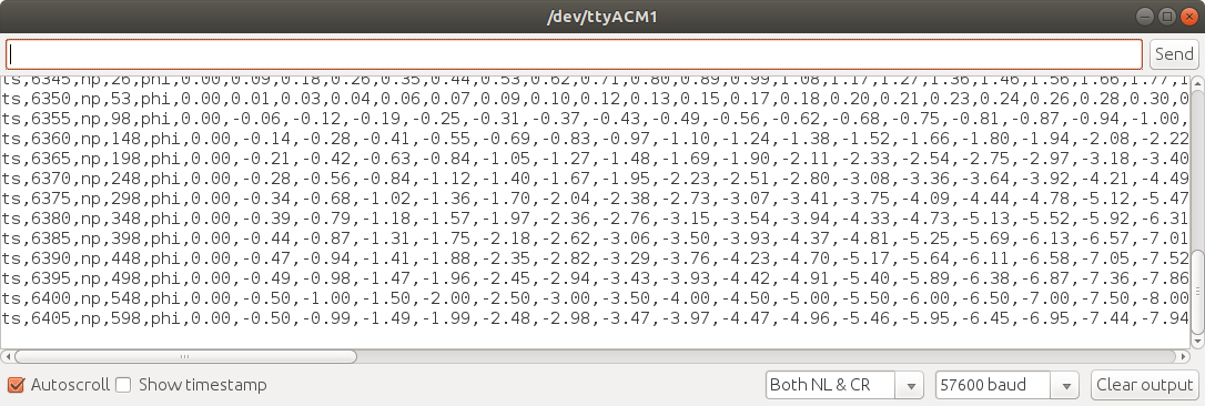
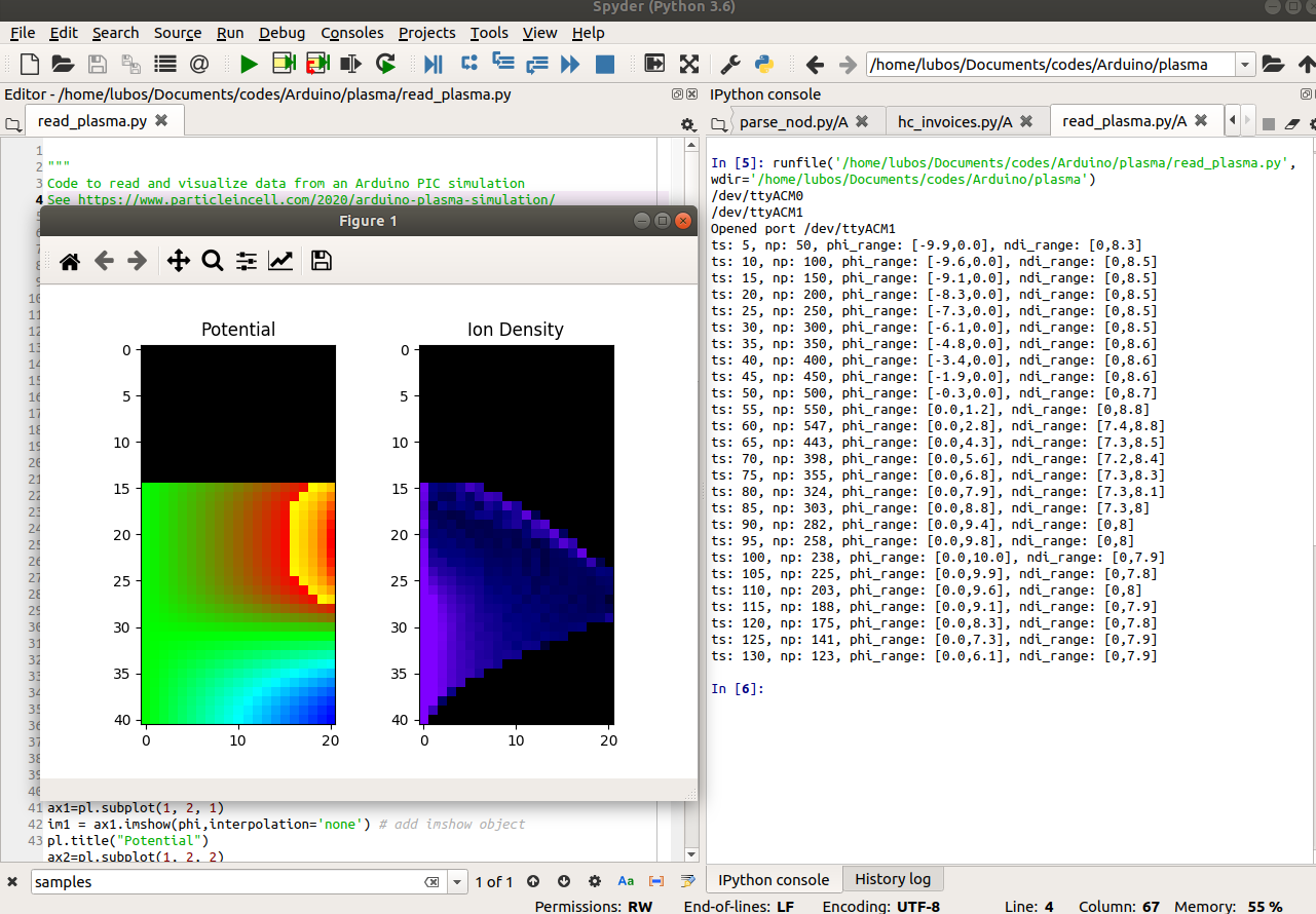
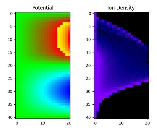
Figure 2 shows the code being uploaded to the microcontroller using the Arduino IDE. The next question you may have is: how to we visualize the results? Just as with other kinetic simulations, we are typically not interested in the state of the individual particles but instead care about the macroscopic fluid properties such as density, stream velocity, or temperature. These values are obtained by scattering particle velocity moments to the grid. Here, we limit ourselves to the density. While we could use a microSD card breakout board to write data to a file, I found it simpler to just communicate the field values over the serial port. This then allowed me to write a Python script to parse the output and animate the simulation in real-time. The output format can be seen in Figure 3. We basically send a text string containing various comma-separated data.
The Python code then basically uses
You can see the video of this animation below:
Figure 6 shows just a single still from the animation in case the video is not working.
Arduino Code
The entire Arduino “plasma.ino” code is copied below:
/*
 * Example hybrid electrostatic Particle-in-Cell (ES-PIC) simulation running on an Arduino
 * More information at https://www.particleincell.com/2020/arduino-plasma-simulation/
 * The code simulates ions moving from left boundary to right where potential oscillates
 * Written by Lubos Brieda, April 2020
 * Tested with MKR Vidor 400
 */

// declare simulation parameters
const float x0 = 0.0;        // mesh origin
const float xm = 0.1;        // mesh extend
const int ni = 21;           // number of nodes
const float dx = xm/(ni-1);  // cell spacing
const float dt = 1e-6;       // time step

const float n0 = 1e9;        // reference number density
const float phi0 = 0;        // reference potential
const float kTe0 = 1;        // reference electron temperature

// physical constants
const float EPS_0 = 8.854187e-12;  // permittivity of free space
const float QE = 1.602e-19;        // elementary charge
const float M = 131*1.660539e-27;  // ion mass, 131 AMU

const int np_max = 1000;           // maximum number of simulation particles
const float w_mp = 1e4;            // macroparticle weight

float* ndi;             // ion number density array
float* phi;             // potential array
float* ef;              // electric field array
float* xp;              // particle positions
float* up;              // particle velocities

unsigned int np = 0;    // actual number of particles
unsigned long ts = 0;   // current time step

// random number generator, returns [0,1)
float rnd() {
  unsigned int rnd_max = 2147483647;
  float r;
  do { r=random(rnd_max)/(float)rnd_max; }
  while (r>=1.0);  // sample again if we get 1.0
  return r;
}

// this is the function that runs when the Arduino is powered up
void setup() {
  Serial.begin(57600);    // open serial port communication
  while(!Serial) {};      // wait for the initialization to complete

  pinMode(LED_BUILTIN, OUTPUT);  // enable writing to the built in LED
  digitalWrite(LED_BUILTIN,0);   // turn off the LED

  ndi = (float*)malloc(ni*sizeof(float));  // allocate memory for ion denstity
  ef = (float*)malloc(ni*sizeof(float));   // allocate memory for electric field
  phi = (float*)malloc(ni*sizeof(float));  // allocate memory for potential

  for (int i=0;i<ni;i++) {
    ndi[i] = 0;   phi[i] = 0;  ef[i] = 0;  // initialize to zero
  }

  xp = (float*)malloc(np_max*sizeof(float)); // allocate memory for ion positions
  up = (float*)malloc(np_max*sizeof(float)); // allocate memory for ion velocities

  for (int i=0;i<10;i++) {                   // blink the LED 10x to update status
    digitalWrite(LED_BUILTIN,0); delay(200);
    digitalWrite(LED_BUILTIN,1); delay(200);
  }

  // optionally, wait to receive 'go' from the serial port before proceeding
  if (0) {
    Serial.println("Done initializing, type 'go' to start");

    while(1) {
      if (Serial.available()>=2) {         // if we have at least two characters
        String str = Serial.readString();  // get the entire string
        Serial.println("read: "+str);      // write out what we received
        if (str[0]=='g' && str[1]=='o') break; // if we get 'g' and 'o', continue
      }
    }
  }

  Serial.println("Starting");   // write to serial port
  digitalWrite(LED_BUILTIN,0);  // turn off LED
}

// this is the code that runs continuosly once setup complets
// it is effective the PIC main loop
void loop() {
  int np_inject = 10;     // number of particles to inject at
  if (np+np_inject>np_max) // check for particle overflow
    np_inject = np_max-np; // adjust particle count if too many

  // inject np_inject particles
  for (int i=0;i<np_inject;i++) {
    xp[np] = x0;
    do {
      up[np] = 10+50*rnd();  // pick random velocity, shoud sample from Maxwellian here!
                             // should also rewind for Leapfrog
    } while(up[np]<0);       // pick again if moving backwards

    np++;                    // update number of particles
  }

  // clear number density array
  for (int i=0;i<ni;i++) {ndi[i] = 0;}

  // scatter particles to the grid to compute number density
  for (int p=0;p<np;p++) {
    float li = (xp[p]-x0)/dx;   // get logical coordinate
    int i = (int)li;            // truncate to get cell index
    float di = li-i;            // fraction distance in the cell
    ndi[i]+= w_mp*(1-di);       // scatter macroparticle weight to the nodes
    ndi[i+1]+=w_mp*(di);
  }

  // divide by cell volume to get number density
  for (int i=0;i<ni;i++) ndi[i]/=dx;
  ndi[0]*=2.0; ndi[ni-1]*=2.0;     // only half-volume on boundaries

  // update potential on the right boundary
  const int freq_ts = 200;
  float f = (ts%freq_ts)/(float)freq_ts;
  phi[0] = 0;
  phi[ni-1] = -10*cos(2*PI*f);

  // compute nonlinear potential, GS for now for simplicity
  for (int k=0;k<100;k++) {   // perform 100 iterations, no convergence check
    for (int i=1;i<ni-1;i++) {
      float rho = QE*(ndi[i] - n0*exp((phi[i]-phi0)/(kTe0))); // charge density
      phi[i] = ((rho/EPS_0)*(dx*dx) + phi[i-1] + phi[i+1])/2; // update potential on node i
    }
  }

  // compute electric field
  ef[0] = (phi[0]-phi[1])/dx;          // one sided difference on left
  ef[ni-1] = (phi[ni-2]-phi[ni-1])/dx; // one sided difference on right
  for (int i=1;i<ni-1;i++)
    ef[i] = (phi[i-1]-phi[i+1])/(2*dx); // central difference everywhere else

  // move particles
  for (int p=0;p<np;p++) {
    float li = (xp[p]-x0)/dx;      // logical coordinate
    int i = (int)li;               // cell index
    float di = li-i;               // fractional distance
    float ef_p = ef[i]*(1-di)+ef[i+1]*(di);  // electric field seen by the particle
    up[p] += QE*ef_p/M*dt;         // update velocity
    xp[p] += up[p]*dt;             // upate position

    if (xp[p]<x0 || xp[p]>=xm) {   // check for particles leaving the domain
      xp[p] = xp[np-1];            // remove particle by replacing with the last one
      up[p] = up[np-1];
      np--;                        // decrease number of particles
      p--;                         // decrement p to recheck this position again
    }
  }

  ts++;  // update time step

  // send field data over the serial port every 5 time steps
  // data sent as ts,999,np,999,phi,999,999,999,...,ndi,999,999,999,...
  if (ts%5==0) {
     String str;
     str="ts,"+String(ts);          // time step
     str+=",np,"+String(np);        // number of particles
     str+=",phi";                   // potential
     for (int i=0;i<ni;i++) str+=","+String(phi[i]);
     str+=",ndi";                   // number density
     for (int i=0;i<ni;i++) str+=","+String(ndi[i]);
     Serial.println(str);           // write out
  }

  /*
  if (ts%100==0) {
    Serial.print(ts);
    Serial.print(":");
    Serial.println(millis()/1000.0);
  }
  */
}
Python visualization code
And here is the Python code used to read the serial port data and animate potential and density. One note, this code is setup to open the Serial port using the Linux device names /dev/ttyACMx where x is a number from 0 to 5. I am not really sure how to open serial port on Windows since all my computers run Linux. Please leave a comment below if you get it working on Windows.
"""
Code to read and visualize data from an Arduino PIC simulation
See https://www.particleincell.com/2020/arduino-plasma-simulation/
Created on Sun Apr 12 22:25:08 2020
@author: Lubos Brieda
"""

import numpy as np
from matplotlib import pyplot as pl
from matplotlib import animation
import serial

# try to find a serial port, this may need to be changed on Windows
# make sure to close Serial Monitor/Plotter in Arduino
port_ok = False
for i in range(0,5):
    try:
        port_name = "/dev/ttyACM%d"%i
        print(port_name)
        ser = serial.Serial(port_name,57600)
        print("Opened port "+port_name)
        port_ok = True
        break
    except serial.SerialException:
        pass

if (not(port_ok)):
    raise Exception("Failed to open port")

ni = 21     # number of nodes in the PIC simulation
nj = 41     # number of rows in time output
L = 10      # some scaling term

rowj=nj     # set current row, we plot from top to bottom
phi = np.zeros((nj,ni,3));  # storage for time data
ndi = np.zeros((nj,ni,3));

fig = pl.figure(1)  # use figure
# equivalent but more general
ax1=pl.subplot(1, 2, 1)
im1 = ax1.imshow(phi,interpolation='none') # add imshow object
pl.title("Potential")
ax2=pl.subplot(1, 2, 2)
im2 = ax2.imshow(ndi,interpolation='none') # repeat for density
pl.title("Ion Density")

def anim(n):
    global rowj
    global phi,ndi
    line = str(ser.readline()); # read line from serial port
    line = line[2:-5]  #eliminate trailing b' and \r\n

    pieces = line.split(','); # split by comma

    if (len(pieces)==(4+2*(1+ni))):  # make sure we get a full line
        ts = float(pieces[1]);  # current time step
        nump = int(pieces[3]);  # number of particles
        if (rowj==0):   # shift down if we reached the bottom
            phi[1:nj,:] = phi[0:nj-1,:]
            ndi[1:nj,:] = ndi[0:nj-1,:]
        else:
            rowj -= 1

        phi_min = 10000    # initialize min/max to get ranges
        phi_max = -10000
        ndi_min = 1e25
        ndi_max = -1e25
        for i in range(ni):
            #[0]='ts', [2]=np,[4]=='phi',[5]=phi0
            phi_val = float(pieces[5+i])  # read potential
            ndi_val = float(pieces[6+ni+i]) # density
            ndi_val = np.log10(max(ndi_val,1)) # convert to log plot

            # update min/max for potential and density
            if (phi_val<phi_min):phi_min = phi_val
            if (phi_val>phi_max):phi_max = phi_val
            if (ndi_val<ndi_min):ndi_min = ndi_val
            if (ndi_val>ndi_max):ndi_max = ndi_val

            # use our RGB functions to convert scalar to [r,g,b]
            phi[rowj,i,:] = rgb1(float(phi_val),-10,10)
            ndi[rowj,i,:] = rgb2(float(ndi_val),7,8)

        # output data range
        print("ts: %d, np: %d, phi_range: [%.1f,%.1f], ndi_range: [%.2g,%.2g]"%(ts,
              nump,phi_min,phi_max,ndi_min,ndi_max))

        # update image
        im1.set_array(phi)
        im2.set_array(ndi)
    return [im1,im2]

# convert to blue-to-red rainbow per
# https://www.particleincell.com/2014/colormap/
def rgb1(val,vmin,vmax):
    f = (val-vmin)/float(vmax-vmin)
    if (f<0): f=0
    if (f>1): f=1

    a=(1-f)*4;
    X=int(a);	  #this is the integer part
    Y=(a-X);   #fractional part from 0 to 255
    if (X==0):
        r=1; g=Y; b=0
    elif (X==1):
        r=1-Y; g=Y; b=0
    elif (X==2):
        r=0; g=1; b=Y
    elif (X==3):
        r=0; g=1-Y; b=1
    else:
        r=0; g=0; b=1

    return [r,g,b];

# convert scalar to shades of purple-blue
def rgb2(val,vmin,vmax):
    f = (val-vmin)/float(vmax-vmin)
    if (f<0): f=0
    if (f>1): f=1
    e Python
    r = max(0.5*(f-0.5)/(1-0.5),0)
    return [r,0,f];

# back in "main", enable animation
anim = animation.FuncAnimation(fig, anim,
                               frames=500, interval=20, repeat=False,blit=False)
pl.show()   # show image
ts: 365, np: 201, phi_range: [-4.3,0.0], ndi_range: [0,8.8]
ts: 370, np: 251, phi_range: [-5.6,0.0], ndi_range: [0,8.8]
ts: 375, np: 301, phi_range: [-6.8,0.0], ndi_range: [0,8.6]
ts: 380, np: 351, phi_range: [-7.9,0.0], ndi_range: [0,8.6]
ts: 385, np: 401, phi_range: [-8.8,0.0], ndi_range: [0,8.5]
ts: 390, np: 451, phi_range: [-9.4,0.0], ndi_range: [0,8.5]
ts: 395, np: 501, phi_range: [-9.8,0.0], ndi_range: [0,8.5]
ts: 400, np: 551, phi_range: [-10.0,0.0], ndi_range: [0,8.5]
ts: 405, np: 601, phi_range: [-9.9,0.0], ndi_range: [0,8.5]
Timing
So just how fast is the Arduino? Given that Arduino code is essentially C, there isn’t much effort needed in porting it to the CPU. We essentially just add a main function that first calls setup(), followed by calling loop() in an infinite loop (or a loop for some given number of steps). In order to eliminate the overhead of serial communication, I “commented out” (by adding 0 && in the if (ts%5==0) condition check) the code outputting serial data, and used
if (ts%1000==0) {
  Serial.print(ts);
  Serial.print(":");
  Serial.println(millis()/1000.0);
}
to write out elapsed time (in seconds) every 1000 time steps.
In the C++ code, besides adding the main function, I also included a class for sampling random numbers, and used <
#include <cstdlib>
#include <iostream>
#include <chrono>
#include <random>

using namespace std;

/* same parameters as in Arduino version */
const float PI = 3.1415926;

// holds starting time
chrono::time_point<chrono::high_resolution_clock> time_start;

// object for sampling random numbers
class Rnd {
public:
  //constructor: set initial random seed and distribution limits
  Rnd(): mt_gen{/*std::random_device()()*/0}, rnd_dist{0,1.0} {}
  void reseed(int seed) {mt_gen.seed(seed);}
  double operator() () {return rnd_dist(mt_gen);}

protected:
  std::mt19937 mt_gen;      //random number generator
  std::uniform_real_distribution<double> rnd_dist;  //uniform distribution
};

Rnd rnd;                    // make an rnd object

// this is the function that runs when the Arduino is powered up
void setup() {
  /* same as Arduino, minus Serial communication and LED blinking */

  //set time start
  time_start =  chrono::high_resolution_clock::now();	//time at simulation start
}

// this is the code that runs continuosly once setup complets
// it is effective the PIC main loop
void loop() {
  /* same as Arduino */
  if (ts%10000==0) {
    auto time_now = chrono::high_resolution_clock::now();
    chrono::duration<double> time_delta = time_now-time_start;
    cout<<ts<<":"<<time_delta.count()<<endl;
  }
}

// main adds the microcontroller loop functionality
int main() {
  setup();
  while(1) {loop();}
  return 0;
}
So what’s the verdict? The Arduino Vidor 4000 took on average 287 seconds per 1000 time steps. The C++ version, built with
g++ -O2 plasma.cpp
running on my 3.2GHz Intel i7-8700 CPU took on average 0.015 seconds per 1000 steps. The Arduino is thus about 20,000x slower than the CPU. But this is not that bad for a tiny board that can run off a battery! And as noted below, it is quite likely that we will be able to obtain additional speedup by developing custom instructions running on the FPGA.
Future Work
So what’s next? Well, the reason I started to look into this board in the first place is due to its on-board FPGA. I plan to soon look into porting some functionality to the FPGA and possibly create a custom FPGA IP library for performing gas-kinetic or fluid simulations. Contact me if interested in collaborating.