USC ASTE-499 Applied Scientific Computing Debrief

In the Spring 2020, I had the opportunity to develop and teach a new course in the Astronautical Engineering Department at University of Southern California. This course was the brainchild of my grad school advisor Prof. Joseph Wang, who is a professor there. His observation, which I strongly agree with, is that the majority of engineering students only learn programming within the realms of MATLAB. While MATLAB is a perfectly fine tool for algorithm prototyping, it is simply inadequate for large-scale simulations, especially those that cannot be easily formulated in terms of matrix equations (as is the case with particle-based methods). Since MATLAB is a weakly typed interpreted language, students also don’t learn such basic programming concepts such as variable types or dynamic memory allocation. For this reason, many professors have to spend a half of semester teaching programming fundamentals instead of focusing on the physics and numerical methods of their respective numerical simulations class. The objective of this course was to introduce students to the wide range of programming languages, as well as hardware architectures and numerical schemes at their disposal. Just as it is extremely helpful to know multiple languages for traveling, I believe it is critical to be a programming polyglot. This way, one can select the best programming language and hardware architecture for the job.
We initially started discussing the course in the Fall of 2018, with the idea that it will be offered first in the Spring and then in the Fall of 2019. But it took some time to get the necessary approvals, plus I had a trip to Europe planned for that September to attend IEPC and visit family. Therefore, we settled on the spring 2020 semester. The course syllabus was quite aggressive, but I am happy to report that we actually managed to stay pretty much on schedule and covered all the topics. Yay! Here is what was discussed:
Syllabus
Class 1 (Scientific Computing Crash Course)
We started by covering basic programming concepts such as variable types, functions, loops, input/output, arrays, random numbers, floating point math, compilation and debugging. One neat thing here was that I demonstrated how to generate the sequence 012345689 (note there is no 7) in the following languages: assembly, Basic, Fortran, Pascal, MATLAB, Python, Lua, R, C, C++, CUDA, Java, C#, D, Rust, Haskell, HTML, Javascript, PHP, Perl, and LaTeX. We then developed a simple program to estimate the value of π by picking random numbers. I was happy to get the assembly version working as it’s been decades since the last time I touched this language.
Class 2 (Numerical Integration)
In the second lesson I introduced the Finite Difference and used it to simulate a ball dropped from a height and bouncing on a surface. This code was developed mainly in C++, but we also went over a version in Python and Fortran 90. Here we also learned how to visualize particle traces in Paraview.
Class 3 (Object Oriented Programming)
This lesson introduced concepts from C++ that your typical MATLAB user will be unfamiliar with. I had real doubts about being able to cover all this material in a single lesson but it actually went OK. We went over data encapsulation, inheritance, virtual functions, templates, and operator overloading. We also learned about pointers (everyone’s favorite!), dynamic memory allocation, and standard library storage containers. We used these concepts to generalize the bouncy ball example to support multiple bouncing objects.
Class 4 (Web Technologies)
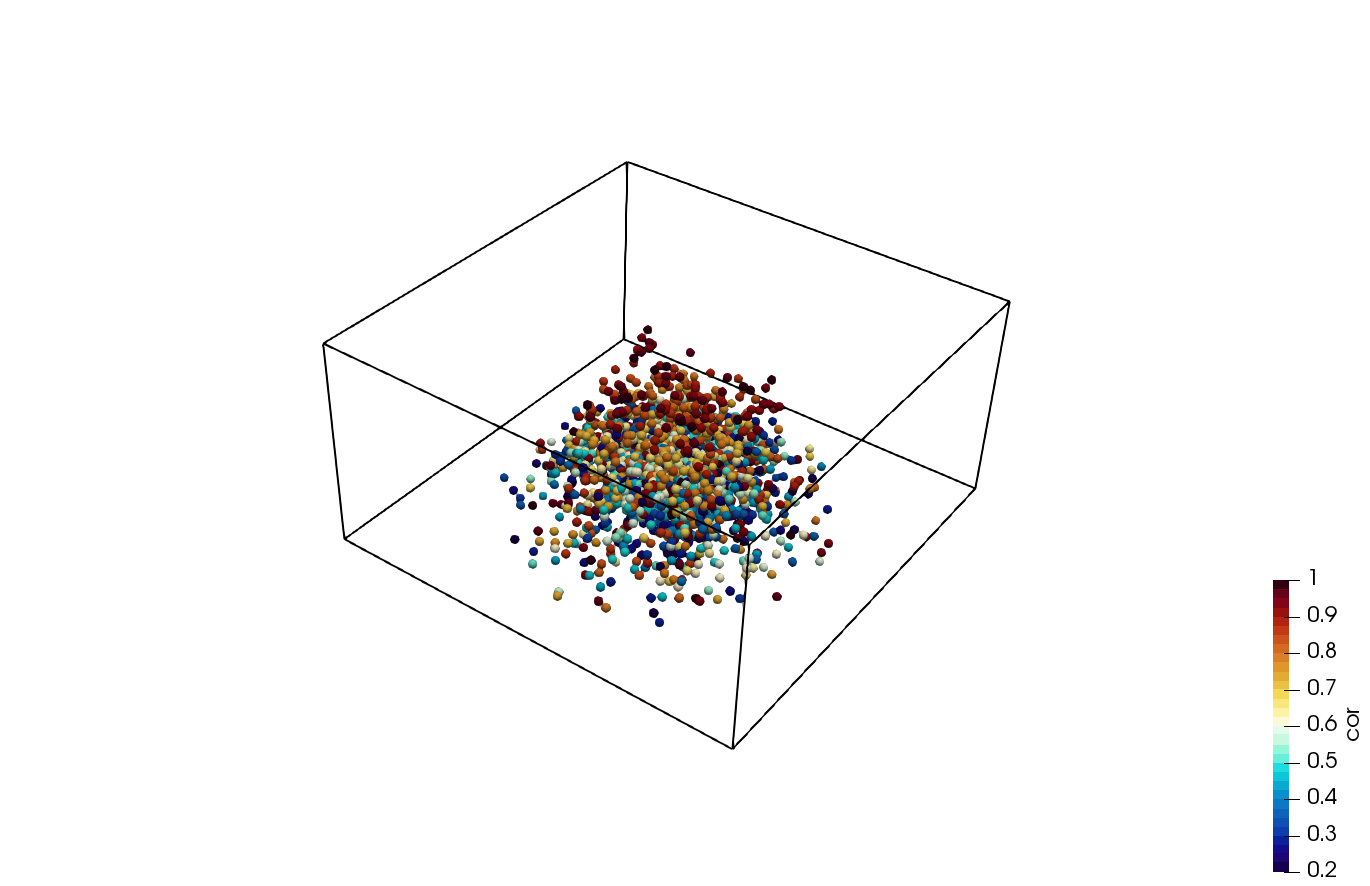
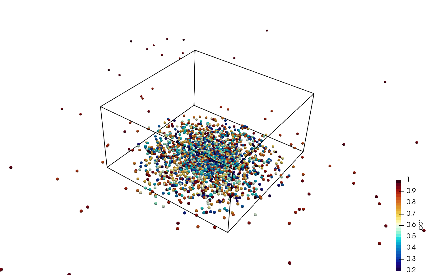
This lesson covered one of my favorite, and seldomly-taught, subject: using Javascript to develop simulation codes that run in a web browser. Not only is this skill useful for “cloud-computing”, it is also not that rare to encounter a computer that does not have a compiler installed. Such may be the case with a lab system used for data acquisition. But since every computer has a web browser, knowing Javascript and a text editor, we can quickly develop code for post-processing data. We started by learning about HTML5 and Javascript. We then developed an interactive version of the bouncy ball program. You can play with it below. The color corresponds to the ball velocity, with mapping per my 2014 colormap article.
Class 5 (Linear Systems)
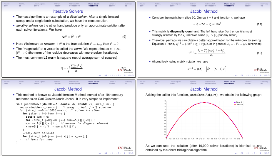
In this lesson, we returned to basics, and covered direct and iterative methods for matrix solving. These methods were not covered in too much detail since it was assumed, at least for this course, that the students have already taken a linear algebra course. We went over Matlab “backslash”, Thomas algorithm, Gauss-Seidel, Multigrid, and Conjugate Gradient algorithms. We also saw how to use Python NumPy and SciPy libraries, and covered memory allocation and access ordering to optimize code performance.
\end{enumerate}
Class 6 (Discretization Schemes)
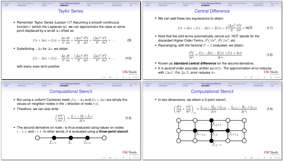
In this lesson we derived the Finite Difference Method (FDM) for 3D applications. We then used it to write a solver for the steady-state diffusion (heat) equation. We also learned how to use Paraview to visualize 3D “image data”.
Class 7 (Fluid Modeling)
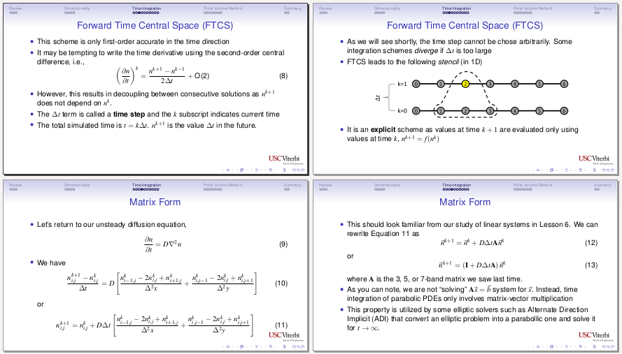
Despte the title, this class was primarily focused on methods for solving unsteady partial differential equations. We introduced the advection diffusion equation as a model for fluid conservation laws, and demonstrated the forward-time, centered space (FTCS) and Crank-Nicolson methods. We also covered models for the advective term and learned about Von Neumann stability analysis. We also went over the Finite Volume method and saw how to use it derive discretization scheme for an axisymmetric problem.
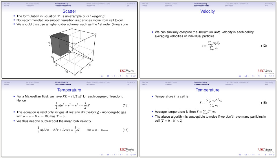
Class 8 (Rarefied Gases)
Next we introduced stochastic Monte-Carlo based methods, specifically Direct Simulation Monte Carlo (DSMC) for modeling rarefied gases. We saw how to obtain macroscopic properties (density, stream velocity, temperature) from the microscopic particle data.
Class 9 (Plasma Simulations)
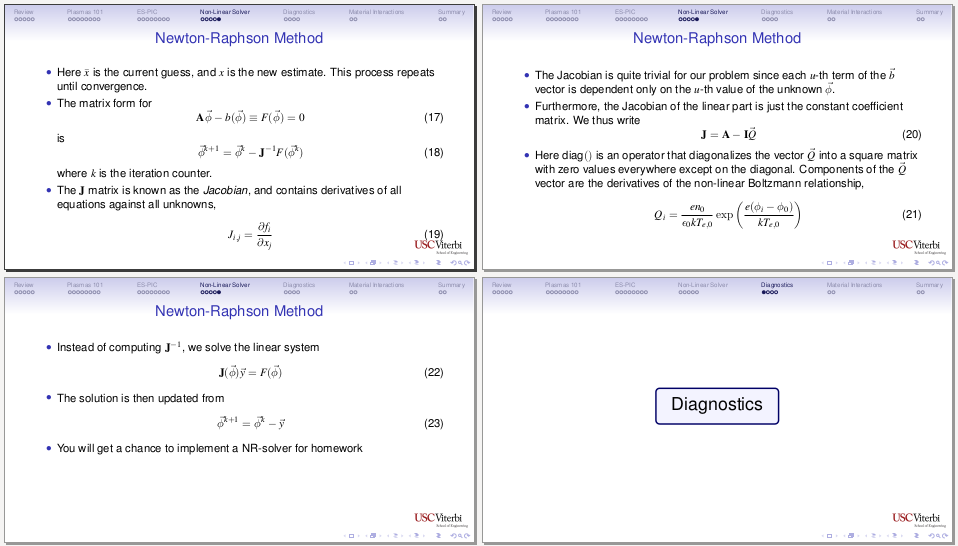
In this lesson we saw how to combine our already-acquired skills (namely, solution methods for the steady-state diffusion/Poisson equation) to add plasma effects via the Electrostatic Particle-in-Cell (ES-PIC)Method. We also went over the Newton-Raphson method for solving non-linear systems. I did not know it at that time, but Class 9 also ended up being the last time I would see my students in person. The students left for spring break after this class, and that is also when the university decided to close the campus and switch to online teaching due to the ongoing COVID-19 pandemic.
Class 10 (Code Testing and Documentation)
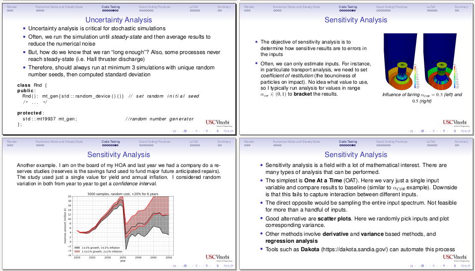
In this lesson, we stepped away from numerical methods and discussed various topics of importance for developing codes that can be used and expanded by others. We went over uncertainty and sensitivity analysis, saw how to use Google Test (GTest) for unit testing, saw how to use Git, and then learned about Doxygen and LaTex for documenting the code and our research.
Class 11 (Multithreading)
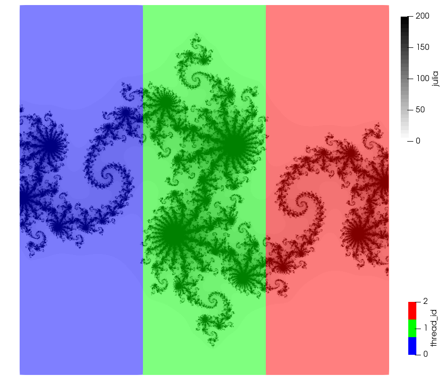
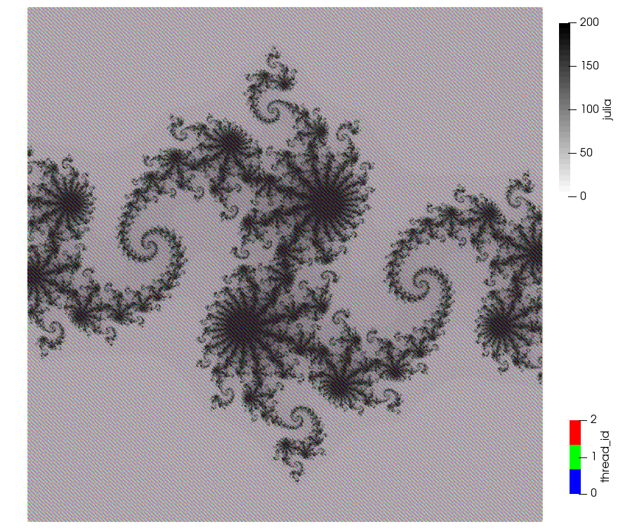
This was the first of 3 lessons introducing high-performance computing. As the title suggests, we started by learning about multithreading. We discussed topics relevant to shared-memory parallelization such as race condition, and how to avoid it without necessarily using locks or mutexes. We also saw, by implementing a parallel version of the Julia set computation, that work assignment distribution is not trivial. By splitting the pixels into blocks, we obtain very poor parallel performance since the middle region in Figure 11 requires much more work than the two boundary ones. By utilizing round-robin strides, we obtain a significant improvement.
Class 12 (Distributed Computing)
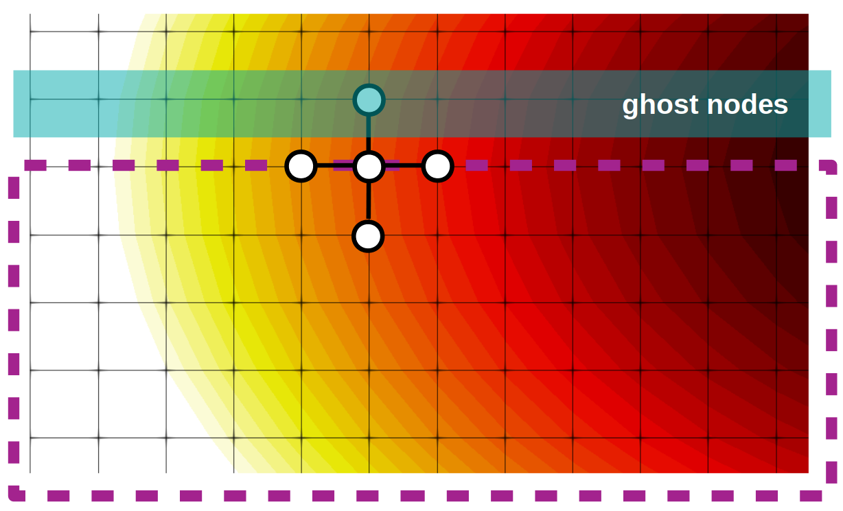
In this second lesson on HPC, we discussed Message Passing Interface (MPI) for developing codes that run on distributed memory clusters. We went over domain decomposition and ensemble averaging are compared. We developed an MPI version of the Julia set code.
Class 13 (GPU programming)
The final lesson on HPC programming covered the use of graphics cards (GPUs). Initially I meant to also include OpenCL, but we ended up focusing solely on CUDA. We discussed performance hit from memory transfer and the use of streams to stack computation and data copy. Since most students did not have computers with an NVIDIA card, we also saw how to create a compute node using Amazon Web Services and how to log onto it and use basic Linux commands to get around. For homework, the students developed a CUDA version of the Julia set code and compared performance to the multithreaded and MPI version. I originally also planned to cover direct rendering with OpenGL but we did not have the time.
Class 14 (Embedded Systems)
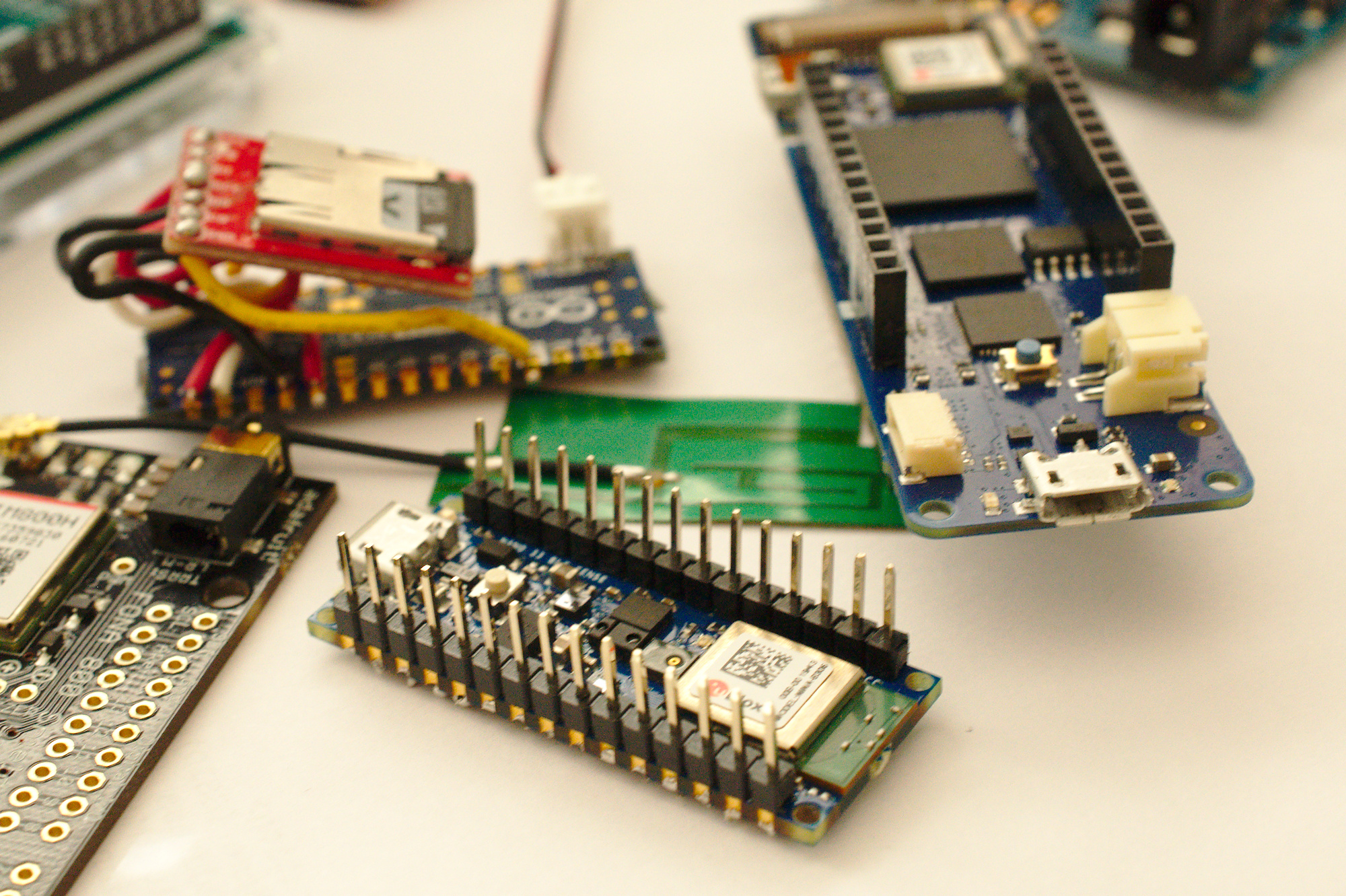
This was one of the lessons I was really looking forward to, which unfortunately ended up being the most difficult one to do over Zoom. The objective here was to introduce the students to hardware-based Arduino and FPGA programming. I was first introduced to Arduinos while working on the water diffusion paper for SPIE. With the knowledge of just a bit of programming and a cheap sensor from DigiKey, Sparkfun, or Adafruit, we can put together data acquisition systems for code validation or other testing that perhaps just a few years would require a massive investment in laboratory equipment. We started by covering different Arduino models, and I then tried to illustrate how to solder on headers onto a breakout board sensor with the help of an USB microscope camera. We also had a quick intro to the Verilog hardware language used to program Field Programmable Gate Arrays (FPGAs).
Class 15 (Optimization and Machine Learning)
In the final lesson, we learned about different parameter optimization strategies including brute force and gradient descent. We then developed a genetic algorithm for the “traveling salesman” problem of finding a shortest round-trip distance among different points (you can play with this code below, although it is not completely bug free). We then discussed deep neural networks and back-propagation for machine learning.
Some Thoughts
As mentioned above, I was quite happy that we managed to get through all these various topics without much of a disaster, given this was the first time teaching this course and most material had to be created from scratch. The main issue for me ended up being finding the time to work on the slides. Slide-making is so time consuming! They were created in LaTeX with the Beamer class, which at least simplified the process of including equations.
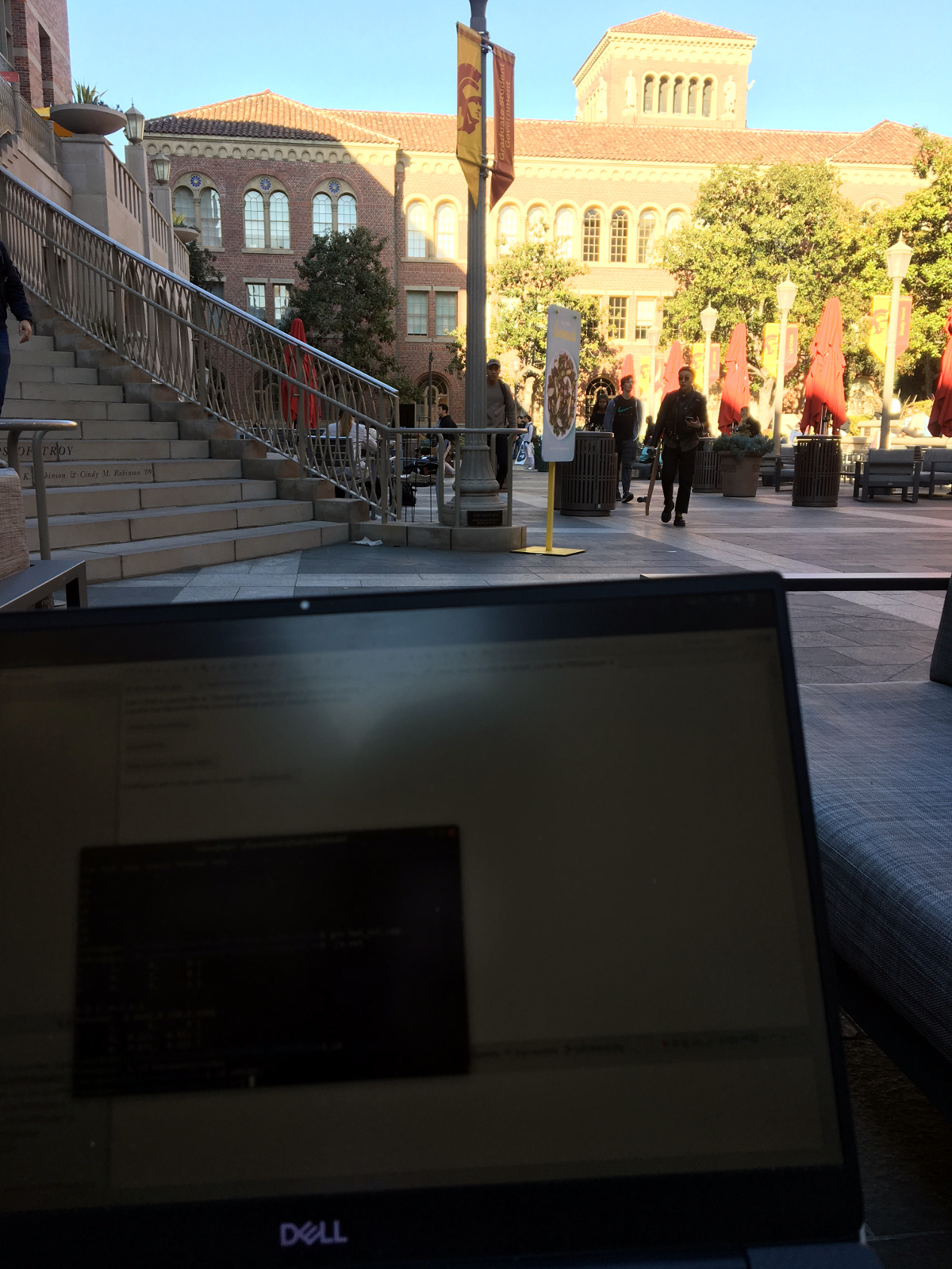
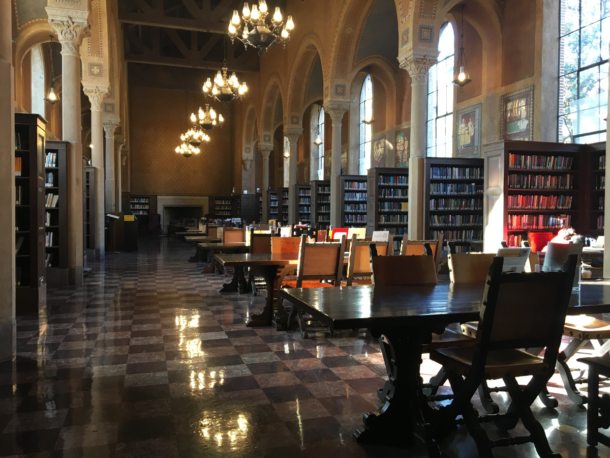
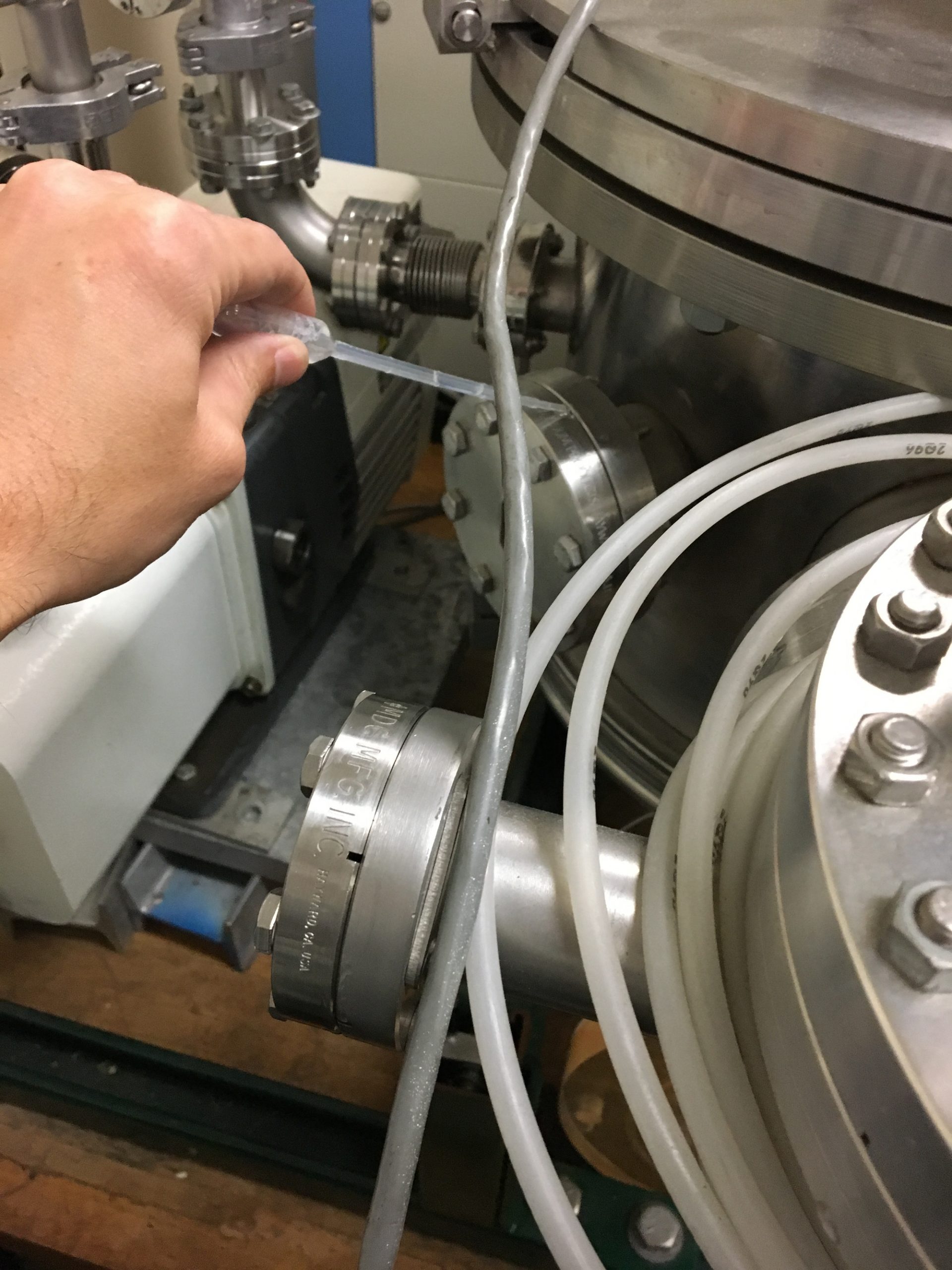
One thing in my favor was that it turns out there is a direct commuter bus from Thousand Oaks to USC that picks up very close to where I live. So at least for the first half of the semester, I ended up with a routine of putting together the examples on Monday, and then using the 2 hour bus ride to organize the draft slides for the lesson. I would continue on these once I got to USC most often in the LiteraTea coffee shop, but sometimes I would also setup in the Ronald Tutor campus center, or the spectacular Hoose Library of Philosophy. I then held an office hour, grabbed a quick snack, and then it was time for my 3 hour lecture. Post lecture, I would head to to Prof. Wang’s lab where I was setting up an experiment to measure outgassing using a Faraday QCM, loaned to use by NASA Goddard, to help validate my CTSP code. Unfortunatelly, just as I was about to install the QCM in the chamber, the pandemic shutdown started. The bus ride back was spent revising the slides, but I generally had to spend another day to finish them and to also put together the homework assignment. In the end, I spent about two solid days on each lesson. In the future, the amount of time needed should be reduced, as much of the material already exists.
On Grading and Attendance
We offered this course as an undergraduate “499” special topics. While this made the approval easier, it also introduced a little wrinkle I was not aware of at first. At USC, or at least in the astronautics department, graduate students are limited to a very small number of 400-level courses they can take for credit. My thinking was that both undergrads and graduate students will be able to take the course, and we just assign more homework to the upper level students (this is what was done for the propulsion course I taught at George Washington). This was not possible, however, and I had several students email me saying they would be interested in taking the course, but also didn’t want to take it if it doesn’t count – and I don’t blame them. Luckily, we still ended up with about 20 registered students in time for Lesson 1. The official minimum to hold a class is 12 so we were in the clear. Quite a few students dropped after this lesson, however, since they probably realized the course isn’t what they were expecting (in case any of them stumble upon this page, I would very much like to hear why!). We then had few more drops but basically held to about 10 students for most of the semester, until about two or three weeks before the end, when we dropped to 6. These students contacted me saying that they were very much enjoying the material but felt they don’t have the time needed to complete the project or the homework assignments. Again, this being an special topics course, I don’t blame them, as I too would prioritize my core classes over an elective. This was also around when the university extended the possibility to withdraw without a penalty until after final grades are posted due to the remote-learning change. The remaining 6 students were really driven to learn the course material, and I was really impressed with every single one of them.
The goal of this course was to introduce a broad spectrum of scientific computing technologies and concepts, and as such, grading was mainly based on weekly homework assignments. These were graded on effort. We also had short “check your understanding” quizzes, and there was a final project. The initial plan was to have students team up into groups to divide the workload, which besides coding also included code documentation and testing. But due to the small class size, most students ended up working on the project alone. The final presentations greatly exceeded my expectations. Some students developed satellite orbit simulators, another student implemented a Discrete Element Method (DEM) particle model in an OpenFOAM simulation, and another group investigated rarefied gas through an orifice using a parallel DSMC code. Finally, I also had each student find some journal or conference paper in their field and do a “book report”. Besides summarizing the numerical method and the results, I was also very interested in having every practice their critical thinking by identifying shortcomings of the chosen approach. The motivation for this type of assignment came from a Biological Nanomachines course taught by Prof. Jonathan Silver at George Washington University. Even though it was outside my field, it ended up being one of the most memorable courses of my Ph.D. study, to a great extent thanks to Prof. Silver’s critical reviews of published work in highly respected journals.
Student Feedback
Of course, in the end, what matters is the student feedback. It came in pretty good, I think, given this was the first time doing this course. Below is what the students had to say:
Is there additional information or feedback that you would like to share with instructor?
- Lectures were extremely well structured – working through coding (especially the C++ programs early on) was very useful to reinforce fundamental concepts such as dynamic data allocation, pointers/references, object–oriented programming, etc. Now that the slides and example scripts are finished, releasing these a few days ahead of each lecture would be very helpful, so students can review material (especially code) beforehand. The classroom setup (multiple screens for code and slides, with a whiteboard to visually work through concepts) also worked great.
- The Homeworks were really good and challenging. Although there were times during the lecture where I felt a bit overwhelmed due to the sheer amount of information. If the lectures were more focused it would be good for me personally.
- Lubos did an excellent job teaching this course! There were some rough edges that come with teaching a special topics course for the first time; which is to be expected. But overall, I found the course to be perhaps the most beneficial course I’ve taken so far in ASTE, at least in the applications to advancing my career technically. The grading for this class was lenient (which is good), but some of the homework assignments were brutal. It’s possible that we went through too much content too quickly. My main feedback for the course is that I think the material could be broadened and split into three courses. The first course could be a 400 level course that looks at the broad range of topics that we discussed in this class. An intro into Python/C++ programming. A look into numerical simulation techniques up to DSMC (not going to PIC), with a case study in particle simulation and something else not related to particle/plasma simulations. And finally a intro to high performance computing (Threading / MPI / GPUs) and optimization (GA’s and ML). I think there could then be two 500 level follow on courses. The first could be more specifically on the topic of plasma/particle simulations. This could take a deeper dive and spend more time expanding on some of the techniques of the first class, and going in to PIC simulations. It could then take more time to investigate high performance computing and optimization as it applies to the field of plasma/particle simulation.The second could be more focused on a different field of modeling and simulation. A class I would love to see is one that looks at larger scale modeling/simulation of space systems. Something that combines previous undergrad/masters coursework on spacecraft design, orbital mechanics, and attitude dynamics/kinematics from a programming / simulation perspective. It too could spend more time expanding on the material of the first class and investigating high performance computing and optimization.
- The scope of this class was really broad and interesting, but sometimes it felt that we were rushing through complex concepts.
- In terms of lecture material, lectures 1–3 and 5–9 (numerical integration, object–oriented programming, discretization schemes, and fluid/particle/plasma modeling) were exceptionally useful in concisely explaining diffuclt topics and were directly applicable to various research topics and engineering disciplines (since they formed the foundation of the material). The multithreading, distributed computing, and GPU lectures were also great additions to the core topics. Homeworks were all extremely useful, as they reinforced topics, making us work through topics discussed in lecture and continue building software started in lecture. As a software class, obviously a large part of the learning process is working through problems and searching out additional information on our own – the assignment definitely facilitated that.
- The programming assignments
- This course got me thinking about difficult and important concepts and applications of computing/numerical methods that I would either not have investigated on my own; or would have struggled to learn on my own. The combination of course material and availability of the instructor to discuss concepts provided a very powerful and beneficial opportunity to learn concepts. The course project got me engaged in topics that I had been interested in for a while but had not had the impetus to get started on learning/exploring.
- Learning parallelization techniques
- Although an interesting topic, the embedded systems lecture was the least useful (only due to the current work–from–home situation) – if we had been in class and able to physically handle hardware, it would have been much more useful. This is also a very broad topic that requires some EE background, but having more detailed explanations of the physics and circuit design behind the embedded systems would have helped (including references for concise books or articles that explain individual components, ie. FPGAs, SOC).
- The course covered quite a few difficult concepts that have broad applications in the field of engineering. Most of these concepts were taught in the context of plasma/particle simulation. This is valuable in it’s own respect, but (for me personally), I would have been interested to see simulation techniques applied to a greater variety of applications.
Please describe the MOST valuable aspect(s) of this course.
Please describe the LEAST valuable aspect(s) of this course.
Next Steps
So what’s next? I am glad for being given this opportunity to teach at USC and am hoping I will be able to continue doing so. Prof. Wang would like to turn this course into a regular part of the Astronautics core curriculum, but this will require splitting it into two courses. The first part will cover basic numerical techniques, algorithm development, and concepts from linear algebra. This undergraduate course will mainly focus on MATLAB and Python, but will also expose students to C++ (and other similar languages) and good coding practices. The follow on graduate course will then introduce advanced topics such as high performance computing, embedded systems, and edge computing. We (along with our collaborator Rob Martin) just submitted a proposal for a new textbook covering these topics. In order to flesh out the material in a bit more detail, I am also considering offering a similar class via my online courses. Let me know by email or a comment below if you would be interested in taking it.