Finite Element Particle in Cell (FEM-PIC)

One of the first articles on this blog was a sample Particle In Cell code on structured Cartesian mesh. In this article, I will try to outline the steps for developing a PIC code that runs on an unstructured mesh. Although I don’t purposely plan to glance over important details, there is much more math going into developing an unstructured code. In fact, the example code was originally developed for the Advanced PIC course, and we spent four lectures and some 200 slides covering the details. Feel free to leave a comment if something is not clear. Or even better, register for the next Advanced PIC course (registration for 2016 course will go live soon)!
Pros and Cons
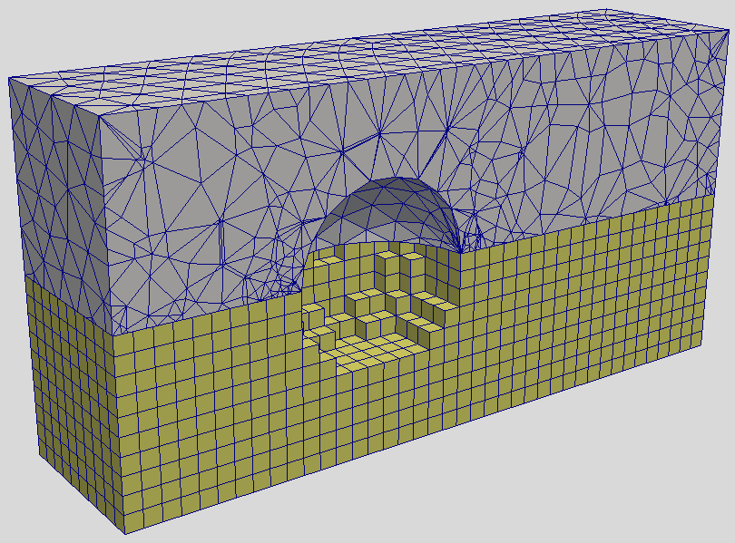
Before getting into the implementation details, I wanted to say few things about pros and cons of unstructured PIC codes. Their primary benefit is the ability to resolve complex geometries. On a Cartesian mesh, we either let the smooth geometry degenerated into a sugar cube representation as shown in Figure 1, or we may develop techniques such as cut-cells. I tried this latter approach in my thesis with mixed results, at best. Unstructured meshes additionally allow us to naturally vary the cell size based on the expected plasma density. Accomplishing something similar with a structured mesh would require adaptive mesh refinement (AMR), leading to a complex mesh description.
Now to the cons. Firstly, particle pushing is much simpler on a structured mesh. This is due to the fact that with a simple (non-AMR) Cartesian mesh, there exists a direct analytical relationship between the particle position and the cell index. Thus, having the particle position, you can easily compute the cell index using relationship such as \(i=(x-x_0)/\Delta x\). No such relationship exists for unstructured meshes. Now each cell has a single index, and the cell index doesn’t have any meaning in regards to its position. In general, we need to find the particle cell by looping through all mesh elements and determining whether a point (the particle) lies within the cell volume. Obviously this is a slow process, given a typical mesh may have tens of thousands of elements. Below I describe a faster algorithm based on neighbor search.
The other drawback is that in the Finite Element Method, the derivative of the solution is available at one less order than the order used in computing the solution. The example posted here uses linear (or first-order) elements. The electric field, the derivative of the potential, is defined only by zeroth-order functions. Zeroth order is a fancy word for constant. Thus, the electric field will be constant in each volume element. This means that as a particle moves from one side of a cell to the order, it does NOT experience a gradual variation in electric field, as is the case with the Finite Difference Method.
Mesh Generation
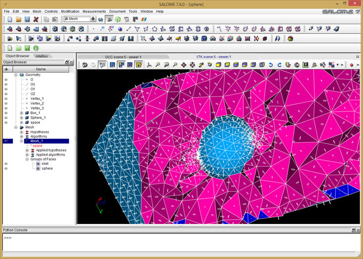
One other difference between structured and unstructured codes is that in the latter case, you also need some way to generate the mesh. In the course, we used Salome, an open source mesher / library platform. The example models flow of ions past a charged sphere. We used Salome’s geometry module to first draw a 3D brick to represent the bounds of the simulation domain. We then used Boolean subtraction to cut a spherical hole in the brick. Next we switched to the meshing module and converted the geometry object into a tetrahedral mesh. This also resulted in creation of triangles on the outer surface. We sorted the triangles into two groups: inlet on the \(z=0\) face, and sphere for triangles on the sphere. This allows us to later set appropriate Dirichlet boundary conditions. Salome supports export in several formats. We used the “dat” format, which is quite simple, but doesn’t support multiple groups in one file. As such, the volume and the two surface mesh groups were exported into three files: mesh.dat, inlet.dat, and sphere.dat.
Mesh Loading
The listing below shows piece of main function of the program. It starts with loading of the volume and surface meshes, exported from Salome.
/**************** MAIN **************************/
int main()
{
	/*instantiate volume*/
	Volume volume;
	if (!LoadVolumeMesh("mesh.dat",volume) ||
	    !LoadSurfaceMesh("inlet.dat",volume,INLET) ||
 	    !LoadSurfaceMesh("sphere.dat",volume,SPHERE)) return -1;
...
}
For example, the surface mesh loader is given below. The surface and volume mesh share same nodes so this code simply loads the node ids and sets the corresponding node to the prescribed type.
/*loads nodes from a surface mesh file and sets them to the specified node type*/
bool LoadSurfaceMesh(const string file_name, Volume &volume, NodeType node_type)
{
	/*open file*/
	ifstream in(file_name);
	if (!in.is_open()) {cerr<<"Failed to open "<<file_name<<endl; return false;}

	/*read number of nodes and elements*/
	int n_nodes, n_elements;
	in>>n_nodes>>n_elements;
	cout<<"Mesh contains "<<n_nodes<<" nodes and "<<n_elements<<" elements"<<endl;

	int nn = volume.nodes.size();

	/*read the nodes*/
	for (int n=0;n<n_nodes;n++)
	{
		int index;
		double x, y, z;

		in >> index >> x >> y >> z;

		if (index<1 || index>nn) {cerr<<"Incorrect node number "<<index<<endl;continue;}
		volume.nodes[index-1].type=node_type;
	}

	cout<<" Done loading "<<file_name<<endl;
	return true;
}
Particle Pusher
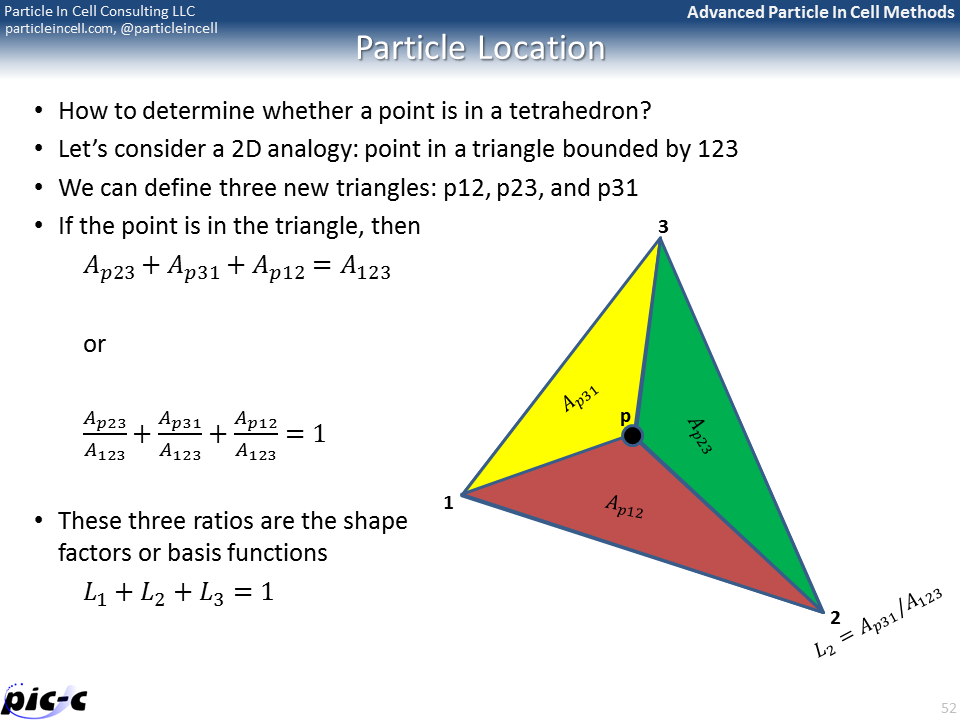
The PIC code needs to know the cell containing each particle so that we can scatter particle densities and also gather electric fields. How do we find the containing cell on a tetrahedral mesh? Let’s consider a 2D analogy: triangular mesh. Imagine you have a triangle 123 as shown in Figure 3 below. Also imagine a particle located at point p. We can subdivide the main triangle into 3 sub-triangles, in which one vertex is replaced by the point p. If p is inside the triangle, \(A_{p23}+A_{p31}+A_{p12}\approx A_{123}\). The approximation is for numerical errors associated with computer arithmetic. Alternatively, we can write \(L_1+L_2+L_3\approx 1\) where \(L_1 \equiv \dfrac{A_{p23}}{A_{123}}\) and so on.
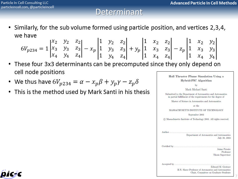
We can do something similar for a tetrahedron. The difference is that since we are now dealing with 3D elements, we need to consider element volumes, not areas. Volume of a tetrahedron is given by a 4×4 determinant. A 4×4 determinant can be rewritten as a linear combination of 3×3 determinants as shown in the second slide in Figure 3. Following thesis of Santi, let point “1” correspond to our particle position and points 2,3,4 be the remaining volume nodes. This then allows us to pre-compute the four 3×3 determinants as they are functions of mesh-geometry only.
Finding the matching cell using a brute force search where we loop over all cells is obviously not computationally feasible. Instead, we can utilize a certain property of the volumes. The sub-volume such as \(V_{p234}\) will be negative if the point is completely behind the face, such 234. We can thus implement the following recursive neighbor search algorithm:
- if inserting a particle for the first time, perform brute force search
- otherwise, check if particle still located in last known cell
- if not, find most negative basis
- check location in the neighbor cell corresponding to this basis
This neighbor search resulted in 43x speed up compared to the brute force for this example mesh. Listing for the XtoL function is given below.
The four basis functions part.lc are used later to scatter particle weights to the mesh.
/*converts physical coordinate to logical, returns true if particle matched to a tet*/
bool XtoLtet(Particle &part, Volume &volume, bool search)
{
	/*first try the current tetrahedron*/
	Tetra &tet = volume.elements[part.cell_index];

	bool inside = true;
	/*loop over vertices*/
	for (int i=0;i<4;i++)
	{
		part.lc[i] = (1.0/6.0)*(tet.alpha[i] - part.pos[0]*tet.beta[i] +
					  part.pos[1]*tet.gamma[i] - part.pos[2]*tet.delta[i])/tet.volume;
		if (part.lc[i]<0 || part.lc[i]>1.0) inside=false;
	}

	if (inside) return true;

	if (!search) return false;
	/*we are outside the last known tet, find most negative weight*/
	int min_i=0;
	double min_lc=part.lc[0];
	for (int i=1;i<4;i++)
		if (part.lc[i]<min_lc) {min_lc=part.lc[i];min_i=i;}

	/*is there a neighbor in this direction?*/
	if (tet.cell_con[min_i]>=0)
	{
		part.cell_index = tet.cell_con[min_i];
		return XtoLtet(part,volume);
	}

	return false;
}
Finite Element Field Solver
The particle pusher is an important part of the FEM-PIC code, but not the only one. The other important piece is the potential solver. Previously, I described the Finite Volume Method which can be used on non-Cartesian meshes. FVM Poisson solver requires secondary control volumes centered on face centroids, which may be difficult to compute for a completely unstructured mesh. For this reason, the Finite Element Method (FEM) is commonly used on unstructured meshes.
The FEM method is quite math heavy, and this section does not come even close to presenting a coherent description. I merely copied several of the 100+ slides used in the course to describe the method. The formulation is based on the Finite Element Method book by Hughes.
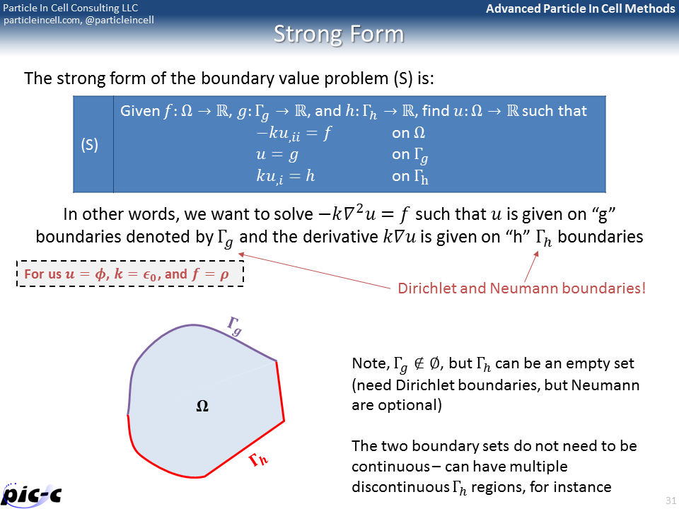
The first slide in Figure 4 shows what’s known as “Strong” form of a boundary value problem. This is the typical formulation, in which the differential equation is given along with a set of Dirichlet and Neumann boundary conditions. The objective is to find the function \(u\). The Finite Element Method is on the other hand based on Weak, or variational, formulation of the problem. This form, defines the problem using several integrals containing test functions (or variations). This weak form can be discretized using element shape functions for the variations, giving us the Galerkin form. This can be further written in a matrix form, giving us the Matrix form, shown in the last slide of Figure 4.

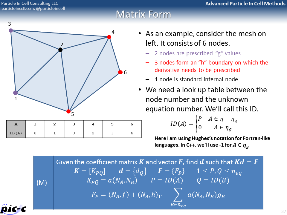
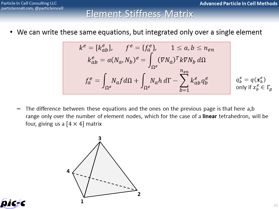
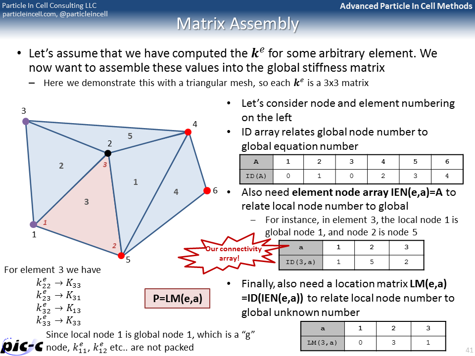
The Matrix form shows that the entire problem reduces to a matrix equation \(Kd=F\), where \(K\) is the global stiffness matrix, \(F\) is the force vector, and \(d\) is the solution vector on the unknown nodes. It is possible to generate the global stiffness matrix by assembling in smaller stiffness matrixes defined for each element. The idea behind this assembly is summarized in Figure 5. The bulk of any FEM code is spent in building the element stiffness matrixes and force vectors, and then assembling them into the right place in the global matrix.

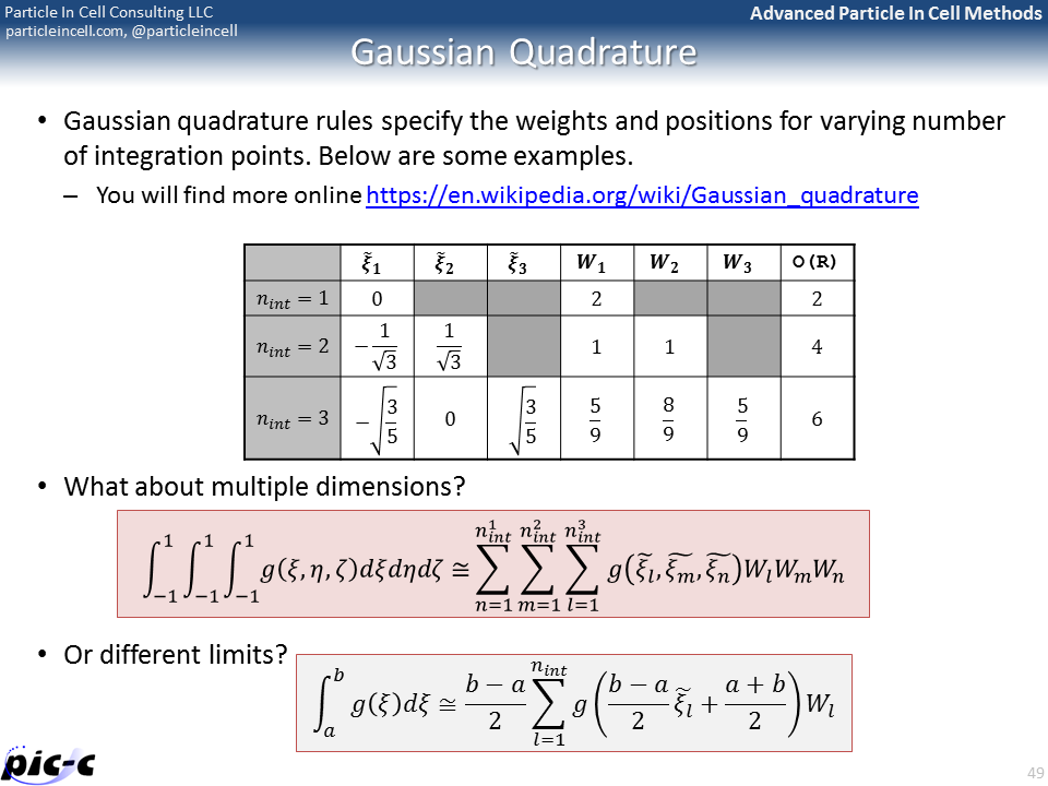
There are many additional details that are still missing. One such a detail is computing integrals from numerical data. The trapezoid rule could be used, but another rule known as Gaussian quadrature is generally superior. It is summarized in the first part of Figure 6. Computing the element stiffness matrix also requires computing derivatives of the shape functions. Part of this process is presented in the second image of Figure 6.

Implementation
As an example, the listing below shows the code used to compute the global K matrix and also pieces of the force vector F that are not dependent on the ion density. That piece is added later, in the Newton-Raphson solver.
/*preassembles the K matrix and "h" and "g" parts of the force vector*/
void FESolver::preAssembly()
{
    /*loop over elements*/
    for (int e=0;e<n_elements;e++)
    {
        Tetra &tet = volume.elements[e];
        double ke[4][4];

        for (int a=0;a<4;a++)
            for (int b=0;b<4;b++)
            {
                ke[a][b] = 0;    /*reset*/

                /*perform quadrature*/
                for (int k=0;k<n_int;k++)
                    for (int j=0;j<n_int;j++)
                        for (int i=0;i<n_int;i++)
                        {
                            double nax[3],nbx[3];

                            double xi = 0.5*(l[i]+1);    /*not used!*/
                            double eta = 0.5*(l[j]+1);
                            double zeta = 0.5*(l[k]+1);
                            getNax(nax,e,a,xi,eta,zeta);
                            getNax(nbx,e,b,xi,eta,zeta);

                            /*dot product*/
                            double dot=0;
                            for (int d=0;d<3;d++) dot+=nax[d]*nbx[d];
                            ke[a][b] += dot*detJ[e]*W[i]*W[j]*W[k];
                        }
            }

        /*we now have the ke matrix*/
        addKe(e,ke);

        /*force vector*/
        double fe[4];

        for (int a=0;a<4;a++)
        {
            /*second term int(na*h), always zero since support only h=0*/
            double fh=0;

            /*third term, -sum(kab*qb)*/
            double fg = 0;
            for (int b=0;b<4;b++)
            {
                int n = tet.con[b];
                double gb = g[n];
                fg-=ke[a][b]*gb;
            }

            /*combine*/
            fe[a] = fh + fg;
        }
        addFe(F0, e,fe);
    }  /*end of element*/
}
The above code is called from main prior to commencing the main loop,
/**************** MAIN **************************/
int main()
{
    /*instantiate volume*/
    Volume volume;
    if (!LoadVolumeMesh("mesh.dat",volume) ||
        !LoadSurfaceMesh("inlet.dat",volume,INLET) ||
        !LoadSurfaceMesh("sphere.dat",volume,SPHERE)) return -1;

    /*instantiate solver*/
    FESolver solver(volume);

    /*set reference paramaters*/
    solver.phi0 = 0;
    solver.n0 = PLASMA_DEN;
    solver.kTe = 2;

    int n_elements = volume.elements.size();
    int n_nodes = volume.nodes.size();

    /*initialize solver "g" array*/
    for (int n=0;n<n_nodes;n++)
    {
        if (volume.nodes[n].type==INLET) solver.g[n]=0;    /*phi_inlet*/
        else if (volume.nodes[n].type==SPHERE) solver.g[n]=-100; /*phi_sphere*/
        else solver.g[n]=0;    /*default*/
    }

    /*sample assembly code*/
    solver.startAssembly();
    solver.preAssembly();    /*this will form K and F0*/

    double dt = 1e-7;

    /*ions species*/
    Species ions(n_nodes);
    ions.charge=1*QE;
    ions.mass = 16*AMU;
    ions.spwt = 2e2;

    /*main loop*/
    int ts;
    for (ts=0;ts<200;ts++)
    {
        /*sample new particles*/
        InjectIons(ions, volume, solver, dt);

        /*update velocity and move particles*/
        MoveParticles(ions, volume, solver, dt);

        /*check values*/
        double max_den=0;
        for (int n=0;n<n_nodes;n++) if (ions.den[n]>max_den) max_den=ions.den[n];

        /*call potential solver*/
        solver.computePhi(ions.den);

        solver.updateEf();

        if ((ts+1)%10==0) OutputMesh(ts,volume, solver.uh, solver.ef, ions.den);

        cout<<"ts: "<<ts<<"t np:"<<ions.particles.size()<<"t max den:"<<max_den<<endl;
    }

    /*output mesh*/
    OutputMesh(ts,volume, solver.uh, solver.ef, ions.den);

    /*output particles*/
    OutputParticles(ions.particles);

    return 0;
}
Results
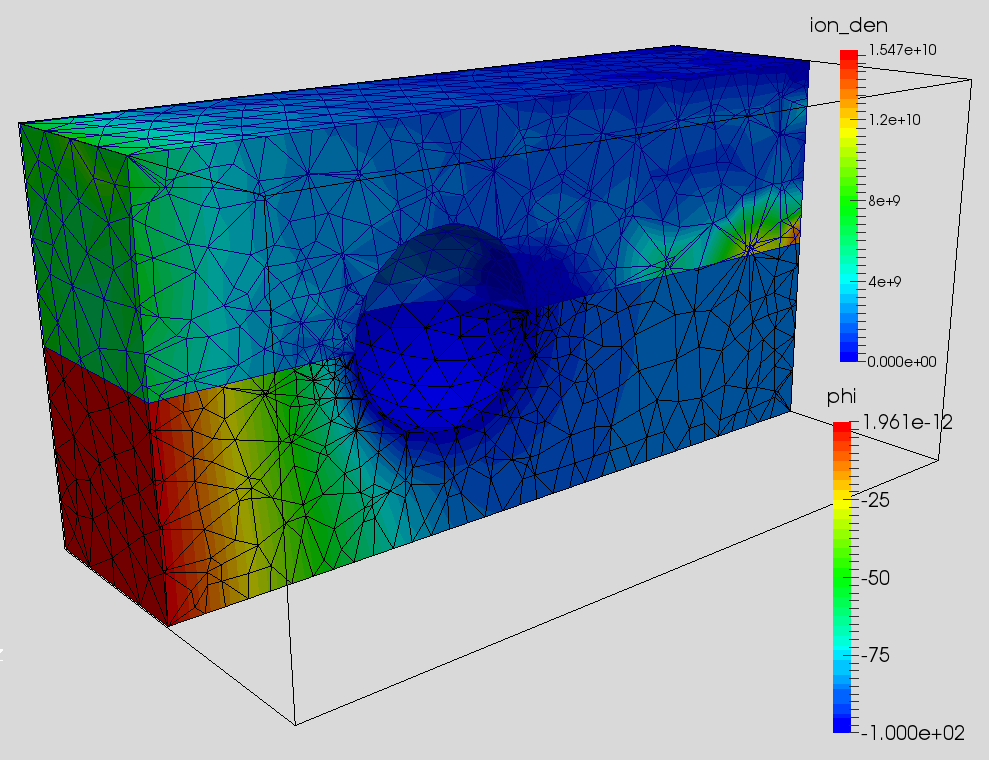
And putting it all together, we end up with a FEM PIC code. Results from the example code are shown below in Figure 7. The first image shows plasma potential and ion density on a center cut. The second image shows an animation of ion density versus time. I have yet to compare these results against the structured PIC code (this same problem is studied in PIC Fundamentals using a Cartesian code), so user beware.

Source Code
You can download the source code here: fem-pic.zip (290kb) or get it from GitHub.
I have yet to do a comparison against the Cartesian code so “use at your risk.” Let me know if you find any bugs.
The code requires a subdirectory called results for storing the VTK files. You can visualize these with Paraview. Use the following to compile and run:
mkdir results
g++ -std=c++11 -O2 fem-pic.cpp -o fem-pic
./fem-pic
References
Hughes, T., “The Finite Element Method: Linear Static and Dynamic Finite Element Analysis”
Hi,
first of all thank you for the blog! It was a very helpful ressource for me.
I am writing a MATLAB code, performing PIC-like calculations ( actually a gun-like raytracing code), that relies on MATLABs pdetool module which makes use of the FEM formalism. On the triangular grid created with pdetool, phi is calculated at the nodes and the electric field at the element centers. Now I have to gather the field to the particles, but do not know which would be a proper interpolation scheme. Linear interpolation from the element centers (where E is defined) seems physically accurate, but creates problems near Neumann boundaries (there are obviously no elements beyond the sim domain). Linear interpolation from cell centers to the respective nodes, before interpolation to the particles violates the Neumann BCs and is per se less accurate due to the use of two interpolations. Would you have any suggestions?
Hi Christoph, assuming you are using 1st-order FEM elements, the derivative (electric field) of the solution (phi) will be given only by zeroth order function. In other words, you only get a single constant value per element. As such, particles see a jump in electric field as they move from cell to cell. This is one big downside of the FEM method. Getting a linearly varying electric field similar to FDM or FVM would require implementing 2nd order elements. Now having said that, many FEM PIC codes are coded up just like this, using constant electric field per element and the results are generally comparable to those from FDM Cartesian codes.
That was the long answer. The short answer is: don’t interpolate.
Hi Lubos,
Thank you for your quick reply (both :-)). I understand why E is defined on the cell only and phi at the nodes, now. However, shouldn’t the scatter & gather parts be programmed equivalent? Because now I perform the trajectory charge scattering to the respective triangular element nodes. Which then results, Matlab internally, to an interpolation from the nodes to the respective cells center of mass, before calculating phi of the next iteration. In short: Shouldn’t I just sum the accumalated trajectory charges to the cells when using 1st order FEM?
No, because scatter and gather need to follow the same basis function as the solution (phi). For first order element this will be the standard area/volume based ratio. It’s only when you get to derivatives that you end up with the constant. By the way, a little plug, I’ll be teaching Advanced PIC in the Fall. About half the course is spent on FEM PIC. As soon as you register, you will have access to the last year’s lecture so you can start reviewing those.
Hi John. I was trying to develop Finite Element Code to model plane truss analysis using MATLAB, please can you show me the way how to do it or can u give me any reference material./Structural Engineering/
Dear Professor:
I am studying the code FEM-PIC, and the code with PLASMA_DEN=1e10, it runs well. But when I set PLASMA_DEN=1e15, the error “GS fails to convergent….”. I study the code, but I do not know why and how to modify.
I need your help.
Thank you very much.
Best Regards.
That is expected. The Poisson solver requires the cell size to be comparable to the Debye length. As you increase the plasma density, you need to correspondingly decrease the cell size. This then in turn makes the Poisson solver approach impractical for real engineering applications since an extremely fine mesh, with millions of cells would need to be used. In the dense region you can instead use the quasineutral assumption and obtain potential by inverting the Boltzmann relationship.
Hi,
First of all I would like to thank you for this material. I have been trying to develop a PIC code and this has been very helpful. I wanted to clarify something though.
In the buildF1Vector function, f(A) is defined as
f(A)=(QE/EPS0)*(ion_den[n]+n0*exp((d[A]-phi0)/kTe)),
but isn’t it supposed to be
f(A)=-(QE/EPS0)*(ion_den[n]-n0*exp((d[A]-phi0)/kTe)).
In that case, the expression for fp_term would also change.
I appreciate you touching on finding a way to generate the mesh with the structured and unstructured codes. My brother is trying to get software that will help with his work project. He needs to find a consultant in the area that is able to help him work through this project on the computer so it’s done properly.