Particle In Cell Method in Cylindrical Coordinates

The first-ever article on this blog was a quick introduction to the Particle In Cell (PIC) Method. That article (and the follow up example) discussed a two-dimensional Cartesian implementation. The ideas presented there are easily extended to 3D codes. But many engineering applications exhibit azimuthal symmetry. For instance, I mainly specialize in electric (i.e. plasma) spacecraft propulsion. Hollow cathodes, used to neutralize the plasma beam, are cylindrical in nature. Similarly, Hall effect thruster (HETs) are also typically studied with two-dimensional axisymmetric codes (although that assumption was brought into question by recent observations of a “rotating spoke” mode at Princeton’s PPPL, see Parker, et. al, APL 97, 091501, 2010, pdf).
Having said all that, how do we go about developing a particle in cell (PIC) code in cylindrical coordinates? This article will show you how.
Differences between XY and RZ codes
Moving from a 3D “xyz” code to a 2D “xy” code is relatively simple. An XY code models a slice through an infinitely deep slab, such plasma flowing around a very long cylinder. Modeling this with a 2D code instead of 3D simply requires using a two-dimensional mesh, and replacing cell volumes with the cell areas, since unit depth can be assumed. Similarly fractional areas are used for scattering and gathering between particles and the mesh.
An RZ code shares similar traits but there are two notable differences: 1) cell volumes grow with distance from the axis of rotation and 2) particle push must take into account the cylindrical geometry.
Problem Setup
To demonstrate the technique, we’ll develop a simulation of a simplistic ion gun. The geometry is shown below in Figure 1. In this example, we’ll use Python with the numPy and sciPy libraries. If you don’t have Python installed yet, the easiest way to get everything in one step, including the Spyder IDE is to download Anaconda.
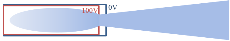
Also, despite calling this method “RZ”, the code is actually “ZR”. The Z axis is the horizontal, and R is the vertical direction. We will refer to “Z” with the “i” index and to “R” with “j”. With this formulation, the third axis is theta, and it points “out of the screen” in the positive direction.
Potential Solver
In the older article on the Finite Volume Method, I showed you how to derive the expression for the Laplacian and gradient in cylindrical coordinates. In summary, we have
$$\nabla^2_R\phi \equiv \frac{\partial^2\phi}{\partial r^2} + \frac{1}{r}\frac{\partial \phi}{\partial r} + \frac{\partial^2\phi}{\partial z^2}$$
where we assumed axial symmetry \(\partial \phi/\partial \theta=0\).
Rewriting the Poisson’s equation using the standard central finite difference, we have
$$\frac{\phi_{i,j+1}-2\phi_{i,j}+\phi_{i,j-1}}{\Delta^2r} + \frac{1}{r_{i,j}}\frac{\phi_{i,j+1}-\phi_{i,j-1}}{2\Delta r} + \frac{\phi_{i-1,j}-2\phi_{i,j}+\phi_{i+1,j}}{\Delta^2z}=-\frac{\rho}{\epsilon_0}$$
To solve this using the Jacobi/Gauss-Seidel method, we simply need to move all non-\(\phi_{i,j}\) terms to the RHS. After a bit of math, we obtain
$$\phi_{i,j}=\left[ \frac{\rho}{\epsilon_0} + \frac{\phi_{i,j+1}+\phi_{i,j-1}}{\Delta^2r}+\frac{1}{r_{i,j}}\frac{\phi_{i,j+1}-\phi_{i,j-1}}{2\Delta r} + \frac{\phi_{i-1,j}+\phi_{i+1,j}}{\Delta^2z}\right]/\left(\frac{2}{\Delta^2r}+\frac{2}{\Delta^2z}\right)$$
We also have the boundary condition
$$\partial \phi/\partial r\Big|_{r=0}=0$$
since there can’t be any sharp change across the axis. This is really just the Neumann boundary condition. In Python, the implementation of the solver may look like this:
for i in range(1,nz-1):
    for j in range(1,nr-1):

    if (cell_type[i,j]>0):
        continue

    rho_e=QE*n0*math.exp((phi[i,j]-phi0)/kTe)
    b = (rho_i[i,j]-rho_e)/EPS0;
    g[i,j] = (b +
             (phi[i,j-1]+phi[i,j+1])/dr2 +
             (phi[i,j-1]-phi[i,j+1])/(2*dr*r[i,j]) +
             (phi[i-1,j] + phi[i+1,j])/dz2) / (2/dr2 + 2/dz2)

    phi[i,j]=g[i,j]
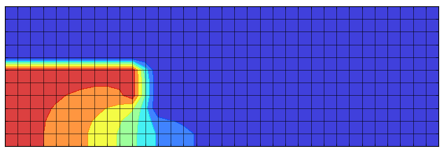
We can alternatively implement the solver using numPy’s vector operators. The solution is shown below in Figure 2. You can see how the potential drop across the aperture optics creates a focusing effect that accelerates the ion beam. This type of configuration is also used to accelerate the ionized propellant in ion thrusters.
#compute electron term
rho_e = QE*n0*numpy.exp(numpy.subtract(P,phi0)/kTe)
b = numpy.where(cell_type<=0,(rho_i - rho_e)/EPS0,0)

#special form along centerline
g[1:-1,0] = (b[1:-1,0] + (phi[2:,0]  + phi[:-2,0])/dz2) / (2/dz2)

#regular form everywhere else
g[1:-1,1:-1] = (b[1:-1,1:-1] +
               (phi[1:-1,2:]+phi[1:-1,:-2])/dr2 +
               (phi[1:-1,0:-2]-phi[1:-1,2:])/(2*dr*r[1:-1,1:-1]) +
               (phi[2:,1:-1] + phi[:-2,1:-1])/dz2) / (2/dr2 + 2/dz2)

#neumann boundaries
g[0] = g[1]       #left
g[-1] = g[-2]     #right
g[:,-1] = g[:,-2] #top

#dirichlet nodes
phi = numpy.where(cell_type>0,P,g)
Electric Field
The electric field in cylindrical coordinates is computed the same way as in Cartesian coordinates, since \(\nabla_R = \nabla_C\).
#computes electric field
def computeEF(phi,efz,efr):
    #central difference
    efz[1:-1] = (phi[0:nz-2]-phi[2:nz+1])/(2*dz)
    efr[:,1:-1] = (phi[:,0:nr-2]-phi[:,2:nr+1])/(2*dr)

    #one sided difference on boundaries
    efz[0,:] = (phi[0,:]-phi[1,:])/dz
    efz[-1,:] = (phi[-2,:]-phi[-1,:])/dz
    efr[:,0] = (phi[:,0]-phi[:,1])/dr
    efr[:,-1] = (phi[:,-2]-phi[:,-1])/dr
Note that this code is not quite correct. It will use the central difference across solid boundaries, but in reality, we should use a one-sided difference. But for the sake of this example, this is sufficient.
Particle Push
Ok, so now we have all we need to compute the forces acting on the particles. But how to actually perform the particle push in cylindrical coordinates? We will do this by pushing the particle in a 3D Cartesian system, but then rotating the particle back to the RZ plane. We retain all three components of velocity. The third components is not \(u_\theta\) but a Cartesian velocity out of the screen, \(u_y\). As such, most particles will end up outside the RZ plane after the push. This is shown graphically in Figure 3. In this notation, “Y” is the perpendicular distance from the plane. “R” (in capital letters) is the radial component of position after the push. The new radial distance, taking into account the movement off the plane is given by the lower case r.
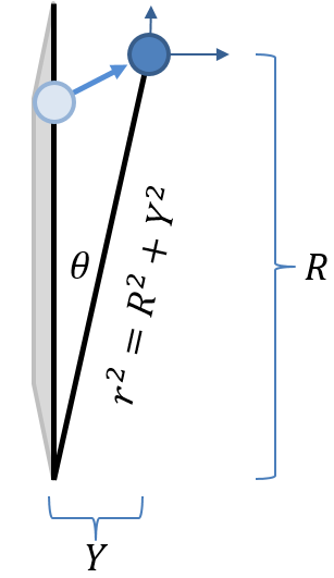
The angle between the RZ plane and the particle position is given by \(\theta_r = \tan^{-1}(Y/R) = \sin^{-1}(Y/r)\). To return the position and velocity back to the RZ plane, we simply need to rotate those two vectors by \(-\theta_r\). Now, since we don’t actually care about “Y” term, we can simplify the algorithm by rotating only the velocity, and replacing particle’s radial position with \(r\). The “rotate to RZ” algorithm is thus
$$ r= \sqrt{R^2+Y^2}$$
and
$$\left[\begin{array}{c}u_r\\u_y\end{array}\right]=\left[\begin{array}{cc}\cos\theta_r & -\sin\theta_r \\ \sin\theta_r & \cos\theta_r\end{array}\right]\left[\begin{array}{c}U_r\\U_y\end{array}\right]$$
The particle push then looks like this:
#push particles
for part in particles:
    #gather electric field
    lc = XtoL(part.pos)
    part_ef = [gather(efz,lc), gather(efr,lc), 0]
    for dim in range(3):
        part.vel[dim] += qm*part_ef[dim]*dt
        part.pos[dim] += part.vel[dim]*dt

    #rotate particle back to ZR plane
    r = math.sqrt(part.pos[1]*part.pos[1] + part.pos[2]*part.pos[2])
    sin_theta_r = part.pos[2]/r
    part.pos[1] = r
    part.pos[2] = 0

    #rotate velocity
    cos_theta_r = math.sqrt(1-sin_theta_r*sin_theta_r)
    u2 = cos_theta_r*part.vel[1] - sin_theta_r*part.vel[2]
    v2 = sin_theta_r*part.vel[1] + cos_theta_r*part.vel[2]
    part.vel[1] = u2
    part.vel[2] = v2
Since we don’t actually need the angle, the code only computes \(\sin \theta_r\) and the cosine is computed from the identity. Also, because of our coordinate system, -pos[2] corresponds to positive sin_theta. But we then need the negative value for the rotation, hence sin_theta_r = part.pos[2]/r = -(-part.pos[2]/r)
Node Volumes
The final change that is required is accounting for the variable node volume. In this axisymmetric code, the simulation cells correspond to an annulus about the centerline. Volume of on annulus centered at node “j” is
$$ V = \pi(r_{j+0.5}^2 – r_{j-0.5}^2)\Delta z$$
For \(j>0\) and constant \(\Delta r\), this formulation is identical to \(2\pi r_j \Delta r \Delta z\), however, the form above makes it more obvious how to compute the node volume at the axis. In the code, we precompute the node volumes and store them in a numPy matrix:
node_volume = numpy.zeros([nz,nr])
for i in range(0,nz):
    for j in range(0,nr):
        j_min = j-0.5
        j_max = j+0.5
        if (j_min<0): j_min=0
        if (j_max>nr-1): j_max=nr-1
        a = 0.5 if (i==0 or i==nz-1) else 1.0
        #note, this is r*dr for non-boundary nodes
        node_volume[i][j] = a*dz*(R(j_max)**2-R(j_min)**2)
Particle Injection: Ionization Model
Even though we have now discussed how to move particles, we still don’t have a way to introduce them into the domain. Since the goal is to model an ion gun, we implement a simple ionization volumetric source. Chemical reactions such as
$$A^0 + e^- \to A^+ + 2e^-$$
can be modeled using rate coefficients,
$$
\begin{align}
\dot{n}_i & = k n_a n_e \\
\dot{n}_e & = k n_a n_e \\
\dot{n}_a & = -k n_a n_e \\
\end{align}
$$
In other words, the rates of increase of ion and electron density are equal and opposite to the rate of decay of the neutral density. In a real device, this reaction results in a “prey and predator” model, where the ionization decreases when neutral density is low, allowing the neutral density (the prey) to rebound. Ionization rate (the predator) then picks up, reducing the neutral density, and hence the ionization rate. Here to keep things simple, I assumed that the electron and neutral densities remain constant. To convert from density increase to the number of macroparticles to inject, simply multiply by cell volume and divide by specific weight. Since this will result in some floating-point number, we use a “remainder” array to store the fractional particles that were not injected and add them to the total at the next sampling. Ions are given a random isotropic velocity. This gives us the following code:
#compute production rate
na = 1e15
ne = 1e12
k = 2e-10  #not a physical value
dni = k*ne*na*dt

#inject particles
for i in range(1,tube_i_max):
    for j in range(0,tube_j_max):

    #skip over solid cells
    if (cell_type[i][j]>0): continue

    #interpolate node volume to cell center to get cell volume
    cell_volume = gather(node_volume,(i+0.5,j+0.5))

    #floating point production rate
    mpf_new = dni*cell_volume/spwt + mpf_rem[i][j]

    #truncate down, adding randomness
    mp_new = int(math.trunc(mpf_new+random()))

    #save fraction part
    mpf_rem[i][j] = mpf_new - mp_new    #new fractional reminder

    #generate this many particles
    for p in range(mp_new):
        pos = Pos([i+random(), j+random()])
        vel = sampleIsotropicVel(300)
        particles.append(Particle(pos,vel))
Results
And that’s it. You can download the entire code from the link below. It runs slow as molasses for me. Since I hardly ever program in Python, it’s possible that there are some obvious (but not to me) ways to speed it up – let me know if you find some! Running the profiler, it appears that most of the computational time is spent in the Gather function.
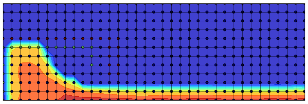
The final ion density is plotted in Figure 4. You can see how the plasma lens accelerates the ion beam. The final ion velocity of ~20km/s agrees reasonably well with the expected 22km/s. The difference is likely due to the ions not having fallen through the entire 100V of potential drop, since they are probably born at locations with potential <100V, and the potential in the plume is slightly higher than 0V.
Source Code
You can download the Python script here: rz-pic.py. Also, I recently started adding the blog examples to Github. You may be interested in cloning the following repo: github.com/particleincell/PICCBlog.
Also, if you would like to learn more about the PIC method, you should sign up for my simulation courses, offered every year.
Perhaps using Numba to autojit the scatter and gather operations might help sir 🙂
Hi Vijai, I am not too familiar with that. Let me know if you try it and get some speed up.
Hey,
thank you for your nice tutorial.
I have one remark: Sometimes it is difficult to use numPy’s vector operators and in this case it is even not the best idea to make the code faster, because there is still a loop (even the biggest one).
In this case, you can use numba.jit() for solving the field which makes it in my case 7 times faster than the vectorized version.
I had nothing to do but taking using loops and write @numba.jit() before function declaration. First time compiling needs like 700 ms, but afterwards it is like 10 ms per calculation.
Best,
Daniel
Thanks for the info, Daniel!
Thanks for the excellent example! Very well put together and easy to follow. I do have a question regarding the node volume calculation however. Why is the node volume not simply dz*(R(j_max)**2-R(j_min)**2)*numpy.pi? Why do you need a=0.5 on the boundaries, don’t the two if statements just above take care of that? And don’t you need that pi in there to get correct numverical results (although not qualitatively different)?
Ah wait, I see know that the factor “a” deals with the boundaries on the z axis while the if statements deal with the boundaries on the r axis. Still confused about the missing factor of pi however.
Hi Grant, that \(\pi\) could be included for “completeness” but it doesn’t change results. Number of particles to create is computed by multiplying ionization rate by dV, and density is later computed by dividing by dV, so any constant scalars just get cancelled out.
So, it is a cartesian to cylindrical code essentially, right?
Changes made to a cartesian code to model cylindrical geometry, if that’s what you mean.
I would like to express the velocities (ux, uy, uz) and positions (x, y, z) to cylindrical coordinates, such as (ur, uf, uz) and (r, f, z). For the (r, f, z) is straightforward. But for velocities are not. All angles with respect to the origin (x, y, z) = (0,0,0)
Hi, interesting article! By the way, isn’t it necessary to modify charge interpolation? Does usage of linear interpolation (the same as in Cartesian 2D) for cylindrical coordinates cause any computation errors?
Yes it is. I have updated this in subsequent codes but haven’t gotten back to updating the article. Thanks for the reminder.